Matrix Transformations and Applications

Introduction

Geometric transformations change the position, orientation, size, or shape of an object.

In coordinate geometry, we can describe these changes using mathematical rules. For example, a rotation through 90° counterclockwise about the origin changes the point (3, 2) into (−2, 3).

Matrices provide a powerful way to represent such transformations.

Instead of applying separate coordinate rules to every point, we can multiply each position vector by a transformation matrix.

Matrix transformations are widely used in:

• Computer graphics and animation

• Video game development

• Architecture and engineering

• Robotics and navigation

• Image processing

• Scientific modelling

In this lesson, we will investigate rotations, reflections, enlargements, stretches, shears, and combinations of transformations. We will also explore how the entries of a matrix determine the geometric effect of a transformation.

Representing Points as Column Vectors

A point P(x, y) can be represented by a column vector:

For example, the point P(3, 2) is represented by:

A two-dimensional linear transformation can be represented by a 2 × 2 matrix:

The transformed point P′ is calculated using:

Multiplying gives:

Therefore:

x′ = ax + by

y′ = cx + dy

These two equations describe how the original coordinates are transformed.

Worked Example: A Simple Transformation

Consider:

Apply A to P(2, 1).

The original point (2, 1) becomes (4, 3).

The x-coordinate has doubled, while the y-coordinate has tripled.

This is a non-uniform stretch.

Visualising Matrix Transformations

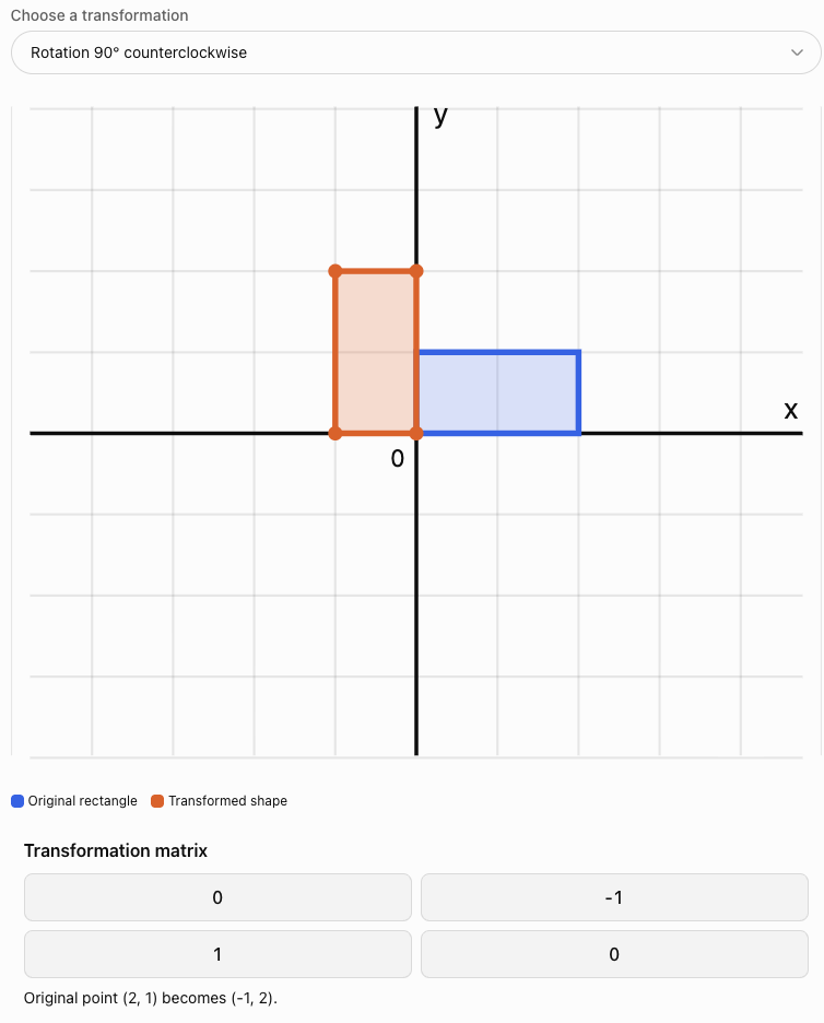
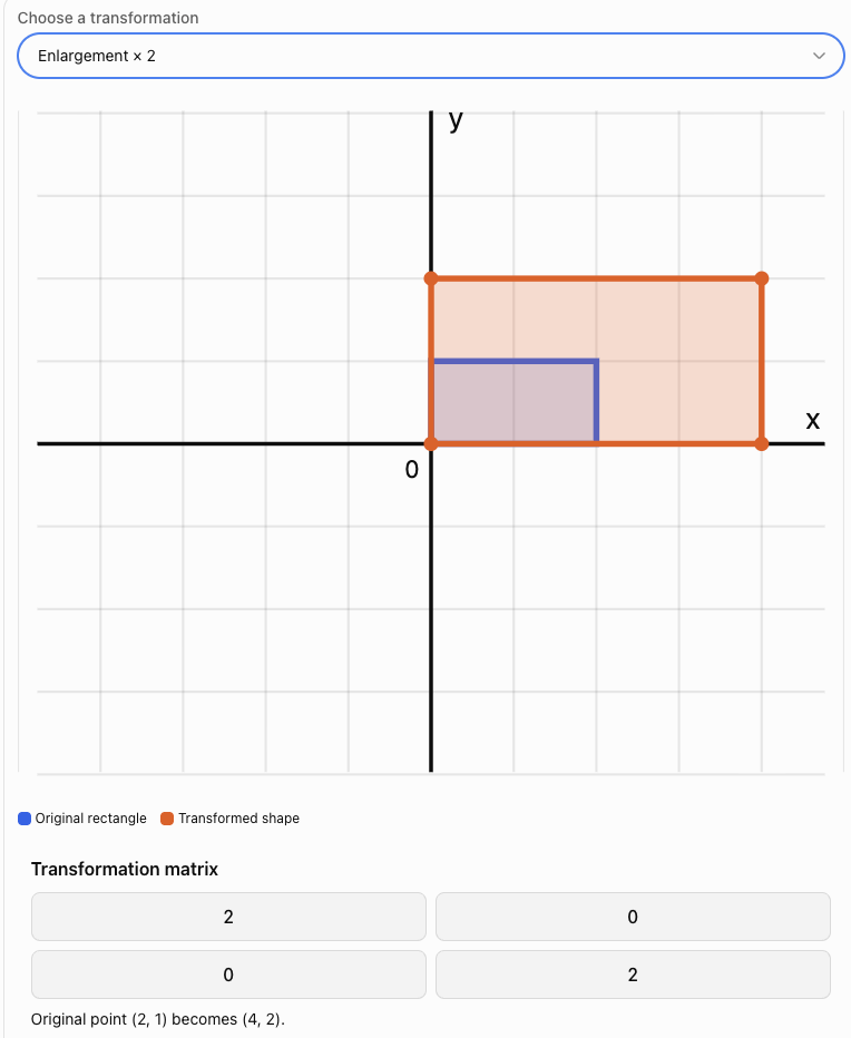
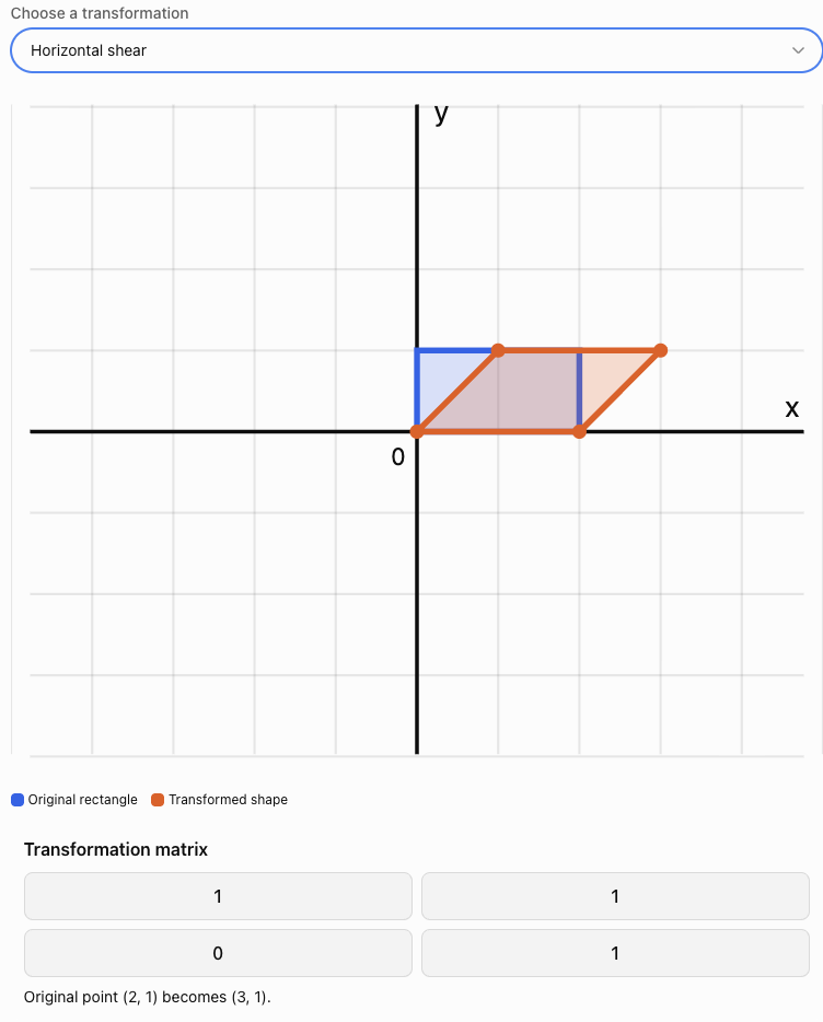
The following interactive explorer shows how a matrix transforms a shape. Change the transformation type to compare the original and transformed shapes.

Rotation Matrices

A rotation turns an object through a specified angle around a fixed point.

For the standard 2 × 2 rotation matrix, the centre of rotation is the origin.

A positive angle represents a counterclockwise rotation.

A negative angle represents a clockwise rotation.

General rotation matrix

For a counterclockwise rotation through an angle θ:

The transformed coordinates are:

x′ = x cos θ − y sin θ

y′ = x sin θ + y cos θ

This formula works for any angle.

Rotation through 90° counterclockwise

Since:

cos 90° = 0

sin 90° = 1

the matrix becomes:

The coordinate rule is:

(x, y) → (−y, x)

Rotation through 180°

Since:

cos 180° = −1

sin 180° = 0

The coordinate rule is:

(x, y) → (−x, −y)

Rotation through 270° counterclockwise

The coordinate rule is:

(x, y) → (y, −x)

This is equivalent to a 90° clockwise rotation.

Summary of common rotation matrices

Worked Example 1: Rotation Through 90°

Rotate P(4, 2) through 90° counterclockwise about the origin.

Step 1: Write the rotation matrix.

Step 2: Write the position vector.

Step 3: Multiply.

x′ = 0(4) − 1(2) = −2

y′ = 1(4) + 0(2) = 4

Therefore:

Verification

The distance from the origin before rotation is:

√(4² + 2²) = √20

After rotation:

√((−2)² + 4²) = √20

The distance remains unchanged.

This is expected because rotations preserve distances.

Worked Example 2: Rotation Through 45°

Rotate P(2, 0) through 45° counterclockwise.

The rotation matrix is:

Multiply:

Therefore:

x′ = √2

y′ = √2

Approximately:

P′ ≈ (1.414, 1.414)

The point remains 2 units from the origin.

Reflection Matrices

A reflection produces a mirror image across a specified line.

Unlike rotations, reflections reverse orientation.

The shape and size remain unchanged.

Reflection in the x-axis

Coordinate rule:

(x, y) → (x, −y)

Reflection in the y-axis

Coordinate rule:

(x, y) → (−x, y)

Reflection in the line y = x

Coordinate rule:

(x, y) → (y, x)

Reflection in the line y = −x

Coordinate rule:

(x, y) → (−y, −x)

Worked Example 3: Reflection in the x-axis

Reflect P(3, 5) in the x-axis.

Therefore:

The x-coordinate remains unchanged, while the y-coordinate changes sign.

Worked Example 4: Reflection in the Line y = x

Reflect the point P(−2, 6) in the line y = x.

The matrix is:

Multiply:

Therefore:

The x- and y-coordinates exchange positions.

Enlargement Matrices

An enlargement changes the size of an object.

For an enlargement with scale factor k about the origin:

The coordinate rule is:

(x, y) → (kx, ky)

Interpreting the scale factor

• k > 1: enlargement

• 0 < k < 1: reduction

• k = 1: identity transformation

• k = 0: collapse to the origin

• k < 0: scaling combined with a 180° reversal in direction

Worked Example 5: Enlargement by Scale Factor 3

Enlarge P(2, −1) by scale factor 3 about the origin.

Therefore:

The distance from the origin becomes three times as large.

The area of any two-dimensional shape becomes 3² = 9 times as large.

Non-Uniform Stretches

A non-uniform stretch changes horizontal and vertical dimensions by different factors.

The general matrix is:

where:

• a is the horizontal scale factor.

• b is the vertical scale factor.

The coordinate rule is:

(x, y) → (ax, by)

Worked Example 6: Horizontal Stretch and Vertical Compression

A rectangle has vertices:

A(0, 0)

B(2, 0)

C(2, 4)

D(0, 4)

Apply:

This stretches horizontally by a factor of 3 and compresses vertically by a factor of 1/2.

The new vertices are:

A′(0, 0)

B′(6, 0)

C′(6, 2)

D′(0, 2)

Original area:

2 × 4 = 8 square units

Transformed area:

6 × 2 = 12 square units

Area scale factor:

12/8 = 1.5

This agrees with:

det(S) = 3(1/2) = 1.5

The determinant describes the signed area scale factor.

Shear Transformations

A shear changes the shape of an object by shifting points parallel to a particular axis.

A square may become a parallelogram.

Unlike an enlargement, a shear does not necessarily change the area.

Horizontal shear

The matrix is:

The coordinate rules are:

x′ = x + ky

y′ = y

Here, k is the shear factor.

A point moves horizontally by an amount proportional to its y-coordinate.

Vertical shear

The matrix is:

The coordinate rules are:

x′ = x

y′ = kx + y

A point moves vertically by an amount proportional to its x-coordinate.

Worked Example 7: Horizontal Shear

Apply the matrix:

to the point P(3, 2).

x′ = 3 + 2(2) = 7

y′ = 2

Therefore:

The point moves 4 units to the right.

Shearing a square

Consider the unit square with vertices:

(0, 0), (1, 0), (1, 1), (0, 1)

Apply a horizontal shear with k = 1.

The new vertices are:

(0, 0), (1, 0), (2, 1), (1, 1)

The square becomes a parallelogram.

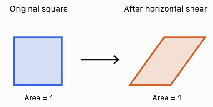
The shear changes the angles but preserves the area.

For a horizontal shear:

det(H) = 1(1) − k(0) = 1

Therefore, the area scale factor is 1.

Combining Transformations

One of the greatest advantages of matrix methods is that several transformations can be combined into a single matrix.

Suppose a point is first transformed by matrix A and then by matrix B.

The first transformation gives:

P′ = AP

The second gives:

P″ = BP′

Substitute:

P″ = B(AP)

Therefore:

The combined transformation matrix is BA, not AB.

The matrix closest to the original vector acts first.

Why order matters

Matrix multiplication is generally not commutative:

AB ≠ BA

Consequently, changing the order of geometric transformations may produce a different result.

Worked Example 8: Reflection Followed by Rotation

A point P(2, 3) is:

1. Reflected in the x-axis.

2. Rotated 90° counterclockwise about the origin.

Find its final coordinates.

Step 1: Write the reflection matrix.

Step 2: Write the rotation matrix.

Step 3: Construct the combined matrix.

Because the reflection happens first:

Combined matrix = RM

Multiplying:

Step 4: Apply the combined transformation.

Therefore:

Geometric interpretation

The combined matrix:

represents a reflection in the line y = x.

Therefore, reflecting in the x-axis and then rotating 90° counterclockwise is equivalent to reflecting in the line y = x.

Worked Example 9: Why Transformation Order Matters

Consider P(1, 2).

Let:

represent a 90° counterclockwise rotation.

Let:

represent a horizontal stretch by factor 2.

Case A: Stretch first, then rotate

The combined matrix is:

RS

Apply to P:

Final point:

(−2, 2)

Case B: Rotate first, then stretch

The combined matrix is:

SR

Apply to P:

Final point:

(−4, 1)

The results are different.

Therefore:

RS ≠ SR

The order of transformations is important.

Interpreting Transformation Matrices Geometrically

A transformation matrix contains information about how the coordinate axes are transformed.

Consider:

The first column:

shows where the unit vector (1, 0) is sent.

The second column:

shows where the unit vector (0, 1) is sent.

This gives a powerful method for understanding any 2 × 2 transformation.

Worked Example 10: Interpreting a Matrix

Consider:

Apply A to the unit vector e₁ = (1, 0):

Apply A to the unit vector e₂ = (0, 1):

Therefore:

• The original horizontal unit vector becomes (2, 0).

• The original vertical unit vector becomes (1, 3).

The unit square becomes a parallelogram with vertices:

(0, 0), (2, 0), (3, 3), (1, 3)

The transformation combines stretching and shearing.

The determinant and area

The determinant is:

det(A) = 2(3) − 1(0)

= 6

Therefore, areas are multiplied by 6.

A unit square with area 1 becomes a parallelogram with area 6.

Determinants and Geometric Transformations

The determinant of a 2 × 2 transformation matrix provides important geometric information.

For:

the determinant is:

det(A) = ad − bc

Geometric meaning

The absolute value of the determinant gives the area scale factor:

The sign of the determinant describes orientation.

Examples

Rotation matrix

det(R) = 1

Rotations preserve area and orientation.

Reflection matrix

det(M) = −1

Reflections preserve area but reverse orientation.

Enlargement by factor k

det(E) = k²

Areas are multiplied by k².

Horizontal shear

det(H) = 1

A shear preserves area and orientation.

Inverse Transformations

An inverse transformation reverses the effect of the original transformation.

If:

P′ = AP

then:

provided A is invertible.

Examples

• The inverse of a 90° counterclockwise rotation is a 90° clockwise rotation.

• The inverse of a reflection is the same reflection.

• The inverse of an enlargement by factor 3 is an enlargement by factor 1/3.

• The inverse of a horizontal shear with factor k is a horizontal shear with factor −k.

Worked Example 11: Reversing a Shear

A point is transformed using:

The transformed point is P′(9, 3).

Find the original point.

Step 1: Find the inverse.

Since det(H) = 1:

Step 2: Apply the inverse.

Therefore:

Transformations About Points Other Than the Origin

Ordinary 2 × 2 matrices describe linear transformations that leave the origin fixed.

However, we may want to rotate or enlarge a shape about another point.

For example, suppose we want to rotate P(x, y) through an angle θ about C(h, k).

We can perform three steps:

1. Translate the centre C to the origin.

2. Apply the rotation.

3. Translate back.

The formula is:

Worked Example 12: Rotation About Another Point

Rotate P(5, 3) through 90° counterclockwise about C(2, 1).

Step 1: Subtract the centre.

P − C = (5 − 2, 3 − 1)

= (3, 2)

Step 2: Rotate through 90°.

(3, 2) → (−2, 3)

Step 3: Add the centre back.

P′ = (−2 + 2, 3 + 1)

Therefore:

Homogeneous coordinates

Translations can also be represented using matrices by introducing a third coordinate.

The point (x, y) becomes:

A translation by (h, k) is represented by:

This method is called homogeneous coordinates.

It is widely used in computer graphics because rotations, translations, stretches, and other affine transformations can then be combined through matrix multiplication.

Real-World Applications

Computer Graphics and Animation

Computer graphics systems use matrices to move, rotate, resize, and distort objects.

A video game character may be represented by thousands of vertices.

Instead of transforming each vertex using separate geometric constructions, the computer applies transformation matrices.

A character can be:

• Rotated to face a new direction.

• Enlarged or reduced.

• Reflected to create a mirrored appearance.

• Sheared to produce visual effects.

• Moved through a scene using homogeneous transformation matrices.

Multiple transformations can be combined into one matrix, improving computational efficiency.

Robotics

Robotic arms contain joints that rotate and move.

Matrices describe how the position of one joint relates to another.

By combining transformation matrices, engineers can calculate the position and orientation of a robot's end effector.

This is important for:

• Manufacturing

• Surgical robotics

• Automated warehouses

• Space exploration

• Precision engineering

Architecture and Engineering

Architects use geometric transformations when creating and modifying designs.

A structural component may need to be rotated, reflected, or scaled.

Shear transformations are also important in understanding how shapes deform under certain loads.

Image Processing

Digital images can be transformed using matrices.

Examples include:

• Rotating photographs

• Reflecting images

• Resizing images

• Correcting perspective

• Creating visual effects

In practical image processing, transformed pixel positions are calculated and image values are resampled to produce the final image.

Common Mistakes

Mistake 1: Multiplying matrices in the wrong order

If A happens first and B second, the combined matrix is BA.

Mistake 2: Confusing clockwise and counterclockwise rotation

A positive angle in the standard rotation matrix means counterclockwise.

Mistake 3: Using row vectors instead of column vectors without adjusting the convention

The matrices in this lesson assume column vectors.

Mistake 4: Forgetting that standard 2 × 2 transformations are about the origin

Transformations about other points require translations or homogeneous coordinates.

Mistake 5: Confusing reflections in the x-axis and y-axis

Reflection in the x-axis changes the sign of y. Reflection in the y-axis changes the sign of x.

Mistake 6: Assuming every transformation preserves area

Rotations, reflections, and standard shears preserve area. Enlargements and non-uniform stretches may change area.

Mistake 7: Confusing scale factor with area scale factor

An enlargement by factor k changes area by k².

Mistake 8: Assuming matrix multiplication is commutative

In general, AB ≠ BA.

Mistake 9: Ignoring the determinant

The determinant gives useful information about area, orientation, and invertibility.

Mistake 10: Assuming every matrix represents a pure rotation or reflection

Some matrices combine several geometric effects.

Mistake 11: Rounding trigonometric values too early

Keep exact values where possible to avoid unnecessary errors.

Mistake 12: Forgetting to transform every vertex

To transform a polygon, apply the matrix to all its vertices.

Key Terms

• Geometric Transformation: Change in the position, orientation, size, or shape of an object.

• Transformation Matrix: Matrix representing a geometric transformation.

• Position Vector: Vector representing a point relative to the origin.

• Image: Result of applying a transformation to a point or shape.

• Preimage: Original point or shape before transformation.

• Rotation: Transformation turning an object through an angle.

• Centre of Rotation: Fixed point around which a rotation occurs.

• Reflection: Transformation producing a mirror image.

• Line of Reflection: Line acting as the mirror.

• Enlargement: Transformation changing an object's size by a scale factor.

• Scale Factor: Number describing how lengths change.

• Uniform Scaling: Scaling equally in every direction.

• Non-Uniform Stretch: Scaling by different factors in different directions.

• Compression: Transformation reducing lengths in a particular direction.

• Shear: Transformation shifting points parallel to an axis by an amount dependent on position.

• Horizontal Shear: Shear that changes x-coordinates.

• Vertical Shear: Shear that changes y-coordinates.

• Composite Transformation: Combination of two or more transformations.

• Identity Matrix: Matrix representing no change.

• Inverse Transformation: Transformation reversing an original transformation.

• Determinant: Scalar describing area scaling, orientation, and invertibility.

• Orientation: Directional ordering of points in a shape.

• Area Scale Factor: Factor by which areas change.

• Singular Matrix: Matrix with determinant zero.

• Unit Vector: Vector of length one.

• Linear Transformation: Transformation preserving vector addition and scalar multiplication.

• Affine Transformation: Transformation combining a linear transformation and translation.

• Homogeneous Coordinates: Coordinate system allowing translations to be represented using matrices.

• Translation: Transformation shifting every point by the same displacement.

• Invariant Point: Point unchanged by a transformation.

Key Takeaways

• Geometric transformations can be represented using matrices.

• A point P is transformed using P′ = AP.

• Rotation matrices use sine and cosine functions.

• A positive rotation angle represents counterclockwise rotation.

• Reflections reverse orientation but preserve distances and area.

• Enlargements change lengths according to a scale factor.

• A uniform enlargement by factor k changes areas by k².

• Non-uniform stretches scale horizontal and vertical dimensions differently.

• Shears change shape while preserving area.

• Composite transformations are calculated using matrix multiplication.

• The order of transformations matters.

• The columns of a transformation matrix show where the coordinate unit vectors are sent.

• The absolute determinant gives the area scale factor.

• A negative determinant indicates reversed orientation.

• An inverse matrix reverses an invertible transformation.

• Transformations about other centres can be handled using translations.

• Homogeneous coordinates allow affine transformations to be combined using matrices.

• Matrix transformations are important in computer graphics, engineering, robotics, and image processing.

Check Your Understanding

Questions

Question 1: Rotation

Rotate P(3, 4) through 90° counterclockwise about the origin.

Question 2: Rotation Through 180°

Rotate P(−5, 2) through 180° about the origin.

Question 3: Reflection in the x-axis

Reflect P(4, −7) in the x-axis.

Question 4: Reflection in y = x

Reflect P(−3, 6) in the line y = x.

Question 5: Enlargement

Enlarge P(2, −4) by scale factor 3 about the origin.

Question 6: Non-Uniform Stretch

Apply:

to P(3, 8).

Question 7: Horizontal Shear

Apply:

to P(2, 4).

Question 8: Vertical Shear

Apply:

to P(3, 1).

Question 9: Combined Transformations

A point is reflected in the x-axis and then rotated through 90° counterclockwise.

Find the combined transformation matrix.

Question 10: Transformation Order

Explain why the order of transformations matters.

Question 11: Determinant and Area

A transformation matrix is:

Determine the area scale factor.

Question 12: Orientation

Determine whether:

preserves or reverses orientation.

Question 13: Inverse Transformation

Find the inverse of:

Question 14: Rotation About Another Point

Rotate P(6, 4) through 90° counterclockwise about C(2, 2).

Question 15: Integrated Challenge

A triangle has vertices:

A(1, 1)

B(3, 1)

C(2, 4)

The triangle is first enlarged by scale factor 2 about the origin and then reflected in the y-axis.

a) Write the enlargement matrix.

b) Write the reflection matrix.

c) Find the combined transformation matrix.

d) Calculate the transformed vertices.

e) Calculate the original and transformed areas.

f) Explain the geometric meaning of the determinant.

Fully Worked Answers

Answer 1: Rotation

A 90° counterclockwise rotation uses:

Answer: (−4, 3)

Answer 2: Rotation Through 180°

A 180° rotation changes the signs of both coordinates.

(−5, 2) → (5, −2)

Answer: (5, −2)

Answer 3: Reflection in the x-axis

The x-coordinate stays the same.

The y-coordinate changes sign.

(4, −7) → (4, 7)

Answer: (4, 7)

Answer 4: Reflection in y = x

The coordinates exchange positions.

(−3, 6) → (6, −3)

Answer: (6, −3)

Answer 5: Enlargement

Scale factor = 3

Multiply both coordinates by 3.

(2, −4) → (6, −12)

Answer: (6, −12)

Answer 6: Non-Uniform Stretch

x′ = 2(3) = 6

y′ = (1/2)(8) = 4

Answer: (6, 4)

Answer 7: Horizontal Shear

x′ = 2 + 3(4) = 14

y′ = 4

Answer: (14, 4)

Answer 8: Vertical Shear

x′ = 3

y′ = 2(3) + 1 = 7

Answer: (3, 7)

Answer 9: Combined Transformations

Reflection in x-axis:

Rotation 90° counterclockwise:

Reflection happens first, so:

Combined matrix = RM

This is equivalent to reflection in y = x.

Answer 10: Transformation Order

Matrix multiplication is generally not commutative.

Therefore:

AB ≠ BA

Applying A first and then B gives BA.

Applying B first and then A gives AB.

These may produce different transformed coordinates.

Answer: The order matters because different transformation sequences can produce different final positions and shapes.

Answer 11: Determinant and Area

det(A) = 3(2) − 1(0)

= 6

Area scale factor = |6|

Answer: 6

Areas become six times as large.

Answer 12: Orientation

det(A) = −1(1) − 0

= −1

The determinant is negative.

Answer: Orientation is reversed.

The transformation is a reflection in the y-axis.

Answer 13: Inverse Transformation

The inverse reverses the stretches.

Answer 14: Rotation About Another Point

Point:

P(6, 4)

Centre:

C(2, 2)

Subtract the centre:

P − C = (4, 2)

Rotate 90° counterclockwise:

(4, 2) → (−2, 4)

Add the centre back:

(−2 + 2, 4 + 2)

Answer: (0, 6)

Answer 15: Integrated Challenge

Original vertices:

A(1, 1)

B(3, 1)

C(2, 4)

Part a: Enlargement matrix

Scale factor = 2

Part b: Reflection matrix

Reflection in the y-axis:

Part c: Combined matrix

Enlargement happens first, then reflection.

Therefore:

Combined matrix = ME

Part d: Transformed vertices

Apply:

(x, y) → (−2x, 2y)

A(1, 1) → A′(−2, 2)

B(3, 1) → B′(−6, 2)

C(2, 4) → C′(−4, 8)

Therefore:

A′(−2, 2), B′(−6, 2), C′(−4, 8)

Part e: Areas

Original triangle:

Base = 3 − 1 = 2

Height = 4 − 1 = 3

Area = 1/2 × 2 × 3

= 3 square units

Transformed triangle:

Base = |−6 − (−2)| = 4

Height = 8 − 2 = 6

Area = 1/2 × 4 × 6

= 12 square units

Area scale factor:

12/3 = 4

Part f: Determinant

The combined matrix is:

det(A) = (−2)(2) − 0

= −4

The absolute determinant is 4, so areas are multiplied by 4.

The negative sign indicates that orientation is reversed.

This agrees with the transformation: enlargement changes area by factor 4, while reflection reverses orientation.

Final Reflection

Matrices provide an efficient and systematic way to describe geometric transformations.

Rotations and reflections change the orientation or position of shapes while preserving their size. Enlargements and stretches change dimensions, while shears alter shape by shifting points in a particular direction.

Combining transformations through matrix multiplication allows complicated geometric operations to be represented by a single matrix.

The order of multiplication is essential because transformations generally do not commute.

The determinant provides a further connection between algebra and geometry, describing area scaling, orientation, and whether a transformation can be reversed.

These ideas form an important foundation for computer graphics, robotics, engineering, and advanced geometry.

The central idea is that a transformation matrix encodes a geometric rule, allowing points and entire shapes to be transformed, combined, analysed, and reversed using matrix operations.