Introduction to Matrices
4. Inverse Matrices
Learning outcomes
- I can calculate inverse matrices.
- I can verify inverse matrices.
- I can solve equations using matrix inverses.
- I can recognise singular matrices.
- I can apply inverse matrices in practical situations.
Introduction
In ordinary arithmetic, many operations can be reversed.
For example, if a number is multiplied by 5, we can reverse the operation by dividing by 5.
5 × 8 = 40
40 ÷ 5 = 8
Matrices have a similar idea. Under certain conditions, a matrix multiplication can be reversed using an inverse matrix.
Suppose a matrix A transforms a vector x into another vector b:
Ax = b
If A has an inverse, we can use that inverse to recover the original vector:
x = A⁻¹b
Inverse matrices are important because they allow us to solve systems of linear equations, reverse geometric transformations, recover original data, and analyse mathematical models.
However, not every matrix has an inverse. Some transformations lose information, making it impossible to recover the original values uniquely.
In this lesson, we will investigate how inverse matrices are calculated, verified, and applied to mathematical and real-world problems.
What Is an Inverse Matrix?
The inverse matrix of a square matrix A is another matrix, written as A⁻¹, that reverses the effect of multiplication by A.
The defining property is:
AA⁻¹ = A⁻¹A = I
where I is the identity matrix.
For a 2 × 2 matrix, the identity matrix is:
The identity matrix plays a role similar to the number 1 in ordinary multiplication.
For example:
5 × 1 = 5
Similarly:
AI = IA = A
Understanding the relationship
If:
Ax = b
then multiplying both sides on the left by A⁻¹ gives:
A⁻¹Ax = A⁻¹b
Since:
A⁻¹A = I
we obtain:
Ix = A⁻¹b
Therefore:
This relationship is fundamental to solving linear systems using matrices.
Visualising inverse transformations
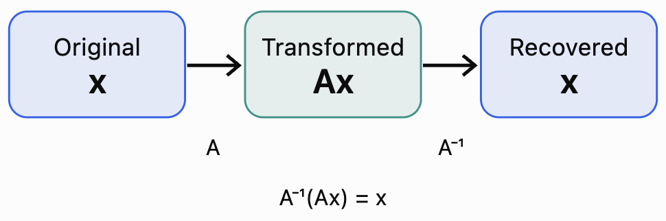
The inverse matrix undoes the original transformation.
Conditions for an Inverse Matrix to Exist
A matrix must satisfy certain conditions before it can have an inverse.
Condition 1: The matrix must be square
A square matrix has the same number of rows and columns.
Examples include:
-
2 × 2 matrices
-
3 × 3 matrices
-
4 × 4 matrices
A rectangular matrix does not have an ordinary two-sided inverse, although some rectangular matrices have specialised one-sided or generalised inverses.
Condition 2: The determinant must not be zero
A square matrix is invertible exactly when:
det(A) ≠ 0
If:
det(A) = 0
the matrix is called singular and does not have an inverse.
Worked Example 1: Checking Invertibility
Consider:
Calculate the determinant:
det(A) = 3(4) − 2(1)
= 12 − 2
= 10
Since det(A) ≠ 0:
A is invertible.
Now consider:
det(B) = 2(6) − 4(3)
= 12 − 12
= 0
Therefore:
B is singular and has no inverse.
Calculating the Inverse of a 2 × 2 Matrix
For a matrix:
the inverse is:
provided:
ad − bc ≠ 0
The four-step method
-
Calculate the determinant: ad − bc.
-
Check that the determinant is not zero.
-
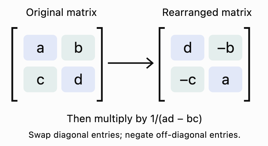
Exchange the positions of a and d, and change the signs of b and c.
-
Multiply every element by 1/det(A).
Visualising the inverse formula
Worked Example 2: Finding an Inverse Matrix
Calculate the inverse of:
Step 1: Calculate the determinant.
det(A) = 4(3) − 1(2)
= 12 − 2
= 10
Step 2: Check invertibility.
Since det(A) = 10 ≠ 0, the inverse exists.
Step 3: Exchange the diagonal elements and change the signs of the other elements.
Step 4: Multiply by 1/10.
Therefore:
Fractions may be preferable when exact answers are required.
Worked Example 3: Inverse with a Negative Determinant
Find the inverse of:
Step 1: Calculate the determinant.
det(B) = 2(4) − 5(3)
= 8 − 15
= −7
Step 2: Apply the inverse formula.
Therefore:
A negative determinant does not prevent a matrix from having an inverse.
Only a zero determinant prevents invertibility.
Verifying Inverse Matrices
Calculating an inverse is only part of the process.
We should also be able to verify that the inverse is correct.
Two square matrices A and B are inverses if:
AB = BA = I
For square matrices of the same order, verifying either AB = I or BA = I is mathematically sufficient, but checking both is useful practice.
Worked Example 4: Verifying an Inverse
Given:
and:
Determine whether B is the inverse of A.
Step 1: Calculate AB.
Top-left:
2(2) + 1(−3) = 1
Top-right:
2(−1) + 1(2) = 0
Bottom-left:
3(2) + 2(−3) = 0
Bottom-right:
3(−1) + 2(2) = 1
Therefore:
Step 2: Calculate BA.
Therefore:
B = A⁻¹
The inverse has been verified.
Interactive Inverse Matrix Explorer
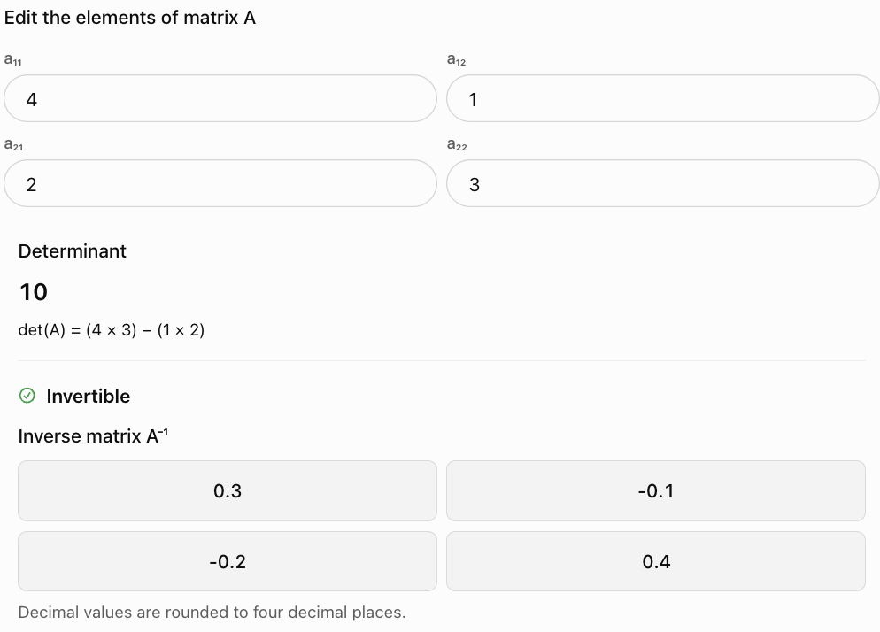
Change the elements of a 2 × 2 matrix to investigate its determinant, inverse, and invertibility.
Finding Inverses Using Row Operations
The 2 × 2 inverse formula is convenient, but larger matrices require more general methods.
One important method is Gauss–Jordan elimination.
This method uses elementary row operations to transform a matrix into the identity matrix.
The augmented matrix method
To find A⁻¹, construct:
[A | I]
Perform row operations until the left side becomes I.
If successful:
[A | I] → [I | A⁻¹]
The right side is then the inverse matrix.
Allowed row operations
-
Swap two rows.
-
Multiply a row by a nonzero scalar.
-
Add a multiple of one row to another row.
Worked Example 5: Inverse Using Gauss–Jordan Elimination
Find the inverse of:
Step 1: Construct the augmented matrix.
Step 2: Swap the two rows.
Step 3: Eliminate the 2 below the first pivot.
R₂ → R₂ − 2R₁
Step 4: Make the second pivot equal to 1.
R₂ → −R₂
Step 5: Eliminate the 1 above the second pivot.
R₁ → R₁ − R₂
The left side is now the identity matrix.
Therefore:
This method works for invertible square matrices of any order.
Finding the Inverse of a 3 × 3 Matrix
A 3 × 3 inverse can be calculated using Gauss–Jordan elimination or the adjugate method.
The general formula is:
where adj(A) is the adjugate matrix, obtained by transposing the matrix of cofactors.
For larger matrices, Gauss–Jordan elimination is often easier to organise.
Worked Example 6: A 3 × 3 Inverse
Find the inverse of:
Start with:
Step 1: Eliminate the 1 in row 2, column 3.
R₂ → R₂ − R₃
Step 2: Eliminate the 1 in row 1, column 2.
R₁ → R₁ − R₂
Therefore:
Verification
Multiplying A by A⁻¹ gives:
The result is the 3 × 3 identity matrix.
Therefore, the inverse is correct.
Solving Matrix Equations Using Inverses
Inverse matrices are especially useful for solving equations of the form:
AX = B
If A is invertible, multiply both sides on the left by A⁻¹:
A⁻¹AX = A⁻¹B
IX = A⁻¹B
Therefore:
Why multiplication order matters
Matrix multiplication is generally not commutative.
Therefore:
A⁻¹B ≠ BA⁻¹
We must multiply on the correct side.
If the original equation is:
XA = B
then:
X = BA⁻¹
provided A is invertible.
Worked Example 7: Solving a Matrix Equation
Solve:
where:
and:
From our earlier example:
Use:
X = A⁻¹B
Calculate the first element:
1(7) + (−1)(4) = 3
Calculate the second element:
(−1)(7) + 2(4) = 1
Therefore:
Verification
The solution is correct.
Solving Systems of Linear Equations
A system of linear equations can be written as a matrix equation.
For example:
2x + 3y = 13
x + 2y = 8
can be written as:
This has the form:
AX = B
Worked Example 8: Solving a System Using the Inverse
Step 1: Identify the coefficient matrix.
Step 2: Calculate the determinant.
det(A) = 2(2) − 3(1)
= 4 − 3
= 1
The inverse exists.
Step 3: Find the inverse.
Step 4: Multiply by the constants.
Therefore:
x = 2
y = 3
Verification
2(2) + 3(3) = 13
2 + 2(3) = 8
Both equations are satisfied.
Solving a System of Three Equations
Inverse matrices can also solve systems with three unknowns.
Consider:
x + y = 5
y + z = 7
z = 4
Write:
From Worked Example 6:
Calculate:
First element:
5 − 7 + 4 = 2
Second element:
7 − 4 = 3
Third element:
4
Therefore:
So:
x = 2, y = 3, z = 4
Singular Matrices
A singular matrix is a square matrix that has no inverse.
A square matrix is singular exactly when its determinant is zero.
Why do singular matrices occur?
Singular matrices often arise when rows or columns are linearly dependent.
For example:
The second column is twice the first column.
The determinant is:
det(A) = 2(6) − 4(3)
= 12 − 12
= 0
Therefore, the matrix is singular.
Geometric interpretation
A singular matrix represents a transformation that collapses space into a lower dimension.
For example, a two-dimensional region may be compressed onto a line.
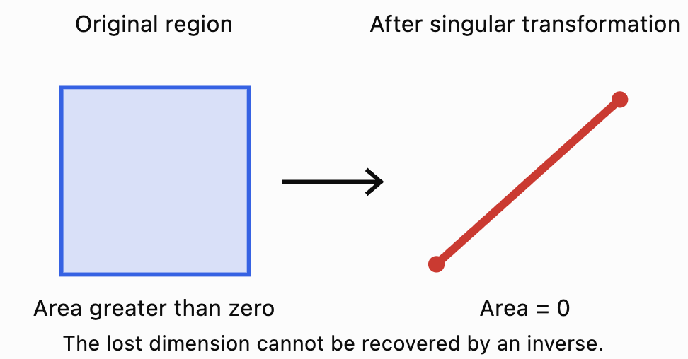
When information is lost in this way, no inverse transformation can uniquely recover every original point.
Singular Matrices and Linear Systems
Consider the system:
2x + 4y = 10
x + 2y = 5
The coefficient matrix is:
Its determinant is:
det(A) = 2(2) − 4(1)
= 0
The matrix is singular.
The first equation is twice the second equation.
Therefore, both equations describe the same line.
There are infinitely many solutions.
Now consider:
2x + 4y = 10
x + 2y = 7
The coefficient matrix is still singular.
However, the equations are inconsistent.
The first equation implies:
x + 2y = 5
while the second requires:
x + 2y = 7
These cannot both be true.
Therefore, the system has no solution.
Important: A zero determinant means that a square linear system does not have a unique solution. It does not tell us whether there are no solutions or infinitely many solutions without examining the equations.
Properties of Inverse Matrices
Inverse matrices follow several useful algebraic rules.
Property 1: Inverse of the inverse
(A⁻¹)⁻¹ = A
Reversing the inverse returns the original matrix.
Property 2: Inverse of a product
(AB)⁻¹ = B⁻¹A⁻¹
The order is reversed.
This is important because matrix multiplication is not generally commutative.
Property 3: Inverse of a transpose
(Aᵀ)⁻¹ = (A⁻¹)ᵀ
Property 4: Inverse of a scalar multiple
For k ≠ 0:
(kA)⁻¹ = (1/k)A⁻¹
provided A is invertible.
Property 5: Identity matrix
I⁻¹ = I
Property 6: Determinant of an inverse
det(A⁻¹) = 1/det(A)
Property 7: Inverse of a power
For a positive integer n:
(Aⁿ)⁻¹ = (A⁻¹)ⁿ
These properties are useful when simplifying complex matrix expressions.
Inverse Matrices and Geometric Transformations
Matrices can represent transformations of points in the coordinate plane.
Inverse matrices reverse these transformations.
Worked Example 9: Reversing a Stretch
Consider:
This transformation stretches x-coordinates by a factor of 2 and y-coordinates by a factor of 3.
For the point:
P(2, 4)
The transformed point is:
The new point is:
P′(4, 12)
To reverse the transformation, calculate the inverse.
Apply the inverse to P′:
The original point has been recovered.
Worked Example 10: Reversing a Rotation
A counterclockwise rotation through 90° is represented by:
The inverse is:
The inverse represents a clockwise rotation through 90°.
If the original point is:
P(3, 2)
the counterclockwise rotation produces:
P′(−2, 3)
Applying R⁻¹ returns:
P(3, 2)
This demonstrates how inverse matrices can undo geometric transformations.
Practical Applications of Inverse Matrices
Application 1: Business and Production Planning
A factory produces two products, A and B.
Each unit of Product A requires:
-
2 hours of machine time.
-
1 hour of labour.
Each unit of Product B requires:
-
1 hour of machine time.
-
3 hours of labour.
The factory has:
-
100 machine hours.
-
120 labour hours.
Let:
x = units of Product A
y = units of Product B
The equations are:
2x + y = 100
x + 3y = 120
Write:
The determinant is:
det(A) = 2(3) − 1(1)
= 5
The inverse is:
Calculate:
Therefore:
The factory should produce 36 units of Product A and 28 units of Product B to use exactly the available machine and labour hours.
Application 2: Recovering Original Data
Suppose two original measurements, x and y, are combined into new measurements:
u = 2x + y
v = x + y
This can be represented as:
If:
u = 11
v = 7
we can recover the original measurements using the inverse.
Therefore:
The original measurements were:
x = 4, y = 3
This type of calculation appears in signal processing and scientific measurement systems.
Application 3: Computer Graphics
Inverse matrices are used in computer graphics to reverse transformations.
For example, a point may be transformed from an object's local coordinate system into a world coordinate system.
An inverse transformation can recover its original local coordinates.
Applications include:
-
Video game graphics
-
Computer animation
-
3D modelling
-
Camera positioning
-
Robotics
-
Engineering simulations
Choosing the Best Method for Finding an Inverse
|
Matrix type |
Recommended method |
|---|---|
|
2 × 2 matrix |
Direct inverse formula |
|
Simple 3 × 3 matrix |
Gauss–Jordan elimination |
|
Larger square matrix |
Row reduction or computational methods |
|
Diagonal matrix |
Take reciprocals of nonzero diagonal elements |
|
Identity matrix |
The inverse is itself |
|
Singular matrix |
No inverse exists |
For a diagonal matrix:
the inverse is:
This works because the diagonal entries are nonzero.
Common Mistakes
Mistake 1: Assuming every matrix has an inverse
Only square matrices with nonzero determinants have ordinary two-sided inverses.
Mistake 2: Dividing every element by the determinant without rearranging the matrix
For a 2 × 2 inverse, the diagonal entries must be exchanged and the off-diagonal signs changed before multiplying by 1/det(A).
Mistake 3: Confusing A⁻¹ with 1/A
Matrix inversion is not element-by-element division.
Mistake 4: Forgetting to check the determinant
If det(A) = 0, the inverse does not exist.
Mistake 5: Making sign errors
Negative signs in the inverse formula must be handled carefully.
Mistake 6: Multiplying matrices in the wrong order
For AX = B:
X = A⁻¹B
not BA⁻¹.
Mistake 7: Assuming AB = BA
Matrix multiplication is generally not commutative.
Mistake 8: Forgetting to verify an inverse
Multiplying A by A⁻¹ should produce the identity matrix.
Mistake 9: Performing row operations on only one side of an augmented matrix
In Gauss–Jordan elimination, every row operation must be applied to the entire augmented matrix.
Mistake 10: Assuming a singular system always has no solution
A singular coefficient matrix may correspond to no solutions or infinitely many solutions.
Mistake 11: Rounding too early
Premature rounding can introduce errors, especially when the determinant is small.
Mistake 12: Forgetting the context of a solution
A mathematical result should be interpreted in the practical situation being modelled.
Key Terms
-
Inverse Matrix: Matrix that reverses the effect of multiplication by an invertible matrix.
-
Invertible Matrix: Square matrix possessing a multiplicative inverse.
-
Identity Matrix: Square matrix with 1 on the main diagonal and 0 elsewhere.
-
Determinant: Scalar value used to determine whether a square matrix is invertible.
-
Singular Matrix: Square matrix with determinant zero.
-
Nonsingular Matrix: Square matrix with nonzero determinant.
-
Matrix Multiplication: Operation combining rows and columns through products and sums.
-
Coefficient Matrix: Matrix containing coefficients of a linear system.
-
Matrix Equation: Equation involving matrices.
-
Augmented Matrix: Matrix formed by placing matrices side by side for row reduction.
-
Elementary Row Operation: Permitted operation used to transform matrix rows.
-
Gauss–Jordan Elimination: Method of row reduction used to solve systems and calculate inverses.
-
Pivot: Leading nonzero element used during row reduction.
-
Row Reduction: Process of simplifying a matrix using elementary row operations.
-
Adjugate Matrix: Transpose of the cofactor matrix.
-
Cofactor: Signed minor associated with a matrix element.
-
Linear Transformation: Mapping represented by matrix multiplication.
-
Inverse Transformation: Transformation that reverses an original transformation.
-
Linear Dependence: Relationship in which one row or column can be expressed using others.
-
Unique Solution: Exactly one solution to a system of equations.
-
Inconsistent System: System with no solutions.
-
Dependent System: System with infinitely many solutions when consistent.
-
Scalar: Single number.
-
Transpose: Matrix formed by interchanging rows and columns.
-
Diagonal Matrix: Square matrix whose off-diagonal entries are zero.
Key Takeaways
-
An inverse matrix reverses the effect of an invertible matrix.
-
The defining property is AA⁻¹ = A⁻¹A = I.
-
Only square matrices with nonzero determinants have ordinary inverses.
-
The inverse of a 2 × 2 matrix can be calculated using a standard formula.
-
The determinant must be checked before calculating an inverse.
-
Inverse matrices can be verified through matrix multiplication.
-
Gauss–Jordan elimination can calculate inverses of larger matrices.
-
Matrix equations of the form AX = B can be solved using X = A⁻¹B.
-
Matrix multiplication order matters.
-
Singular matrices have determinant zero and no inverse.
-
A singular coefficient matrix cannot produce a unique solution to a square linear system.
-
Inverse matrices can reverse geometric transformations.
-
Inverse matrices are useful in business, science, engineering, and computer graphics.
-
In practical problems, solutions must be interpreted in context.
Check Your Understanding
Questions
Question 1: Invertibility
Determine whether the matrix is invertible:
Question 2: Finding an Inverse
Find:
for:
Question 3: Negative Determinant
Find the inverse of:
Question 4: Singular Matrix
Explain why:
has no inverse.
Question 5: Verification
Verify whether:
is the inverse of:
Question 6: Matrix Equation
Solve:
AX = B
where:
Question 7: Linear System
Solve using matrix inverses:
3x + y = 11
x + y = 5
Question 8: Diagonal Matrix
Find the inverse of:
Question 9: Inverse Properties
If det(A) = 5, calculate det(A⁻¹).
Question 10: Product of Inverses
Simplify:
(AB)⁻¹
Question 11: Unknown Matrix Element
Find k so that:
is singular.
Question 12: Geometric Transformation
A transformation doubles x-coordinates and triples y-coordinates.
Write the transformation matrix and its inverse.
Question 13: Three-Variable System
Use the inverse:
to solve:
Question 14: Business Application
A factory makes two products.
Product A requires 2 hours of machine time and 1 hour of labour.
Product B requires 1 hour of machine time and 2 hours of labour.
The factory has 80 machine hours and 70 labour hours.
Use inverse matrices to determine the number of units of each product.
Question 15: Integrated Challenge
Given:
a) Calculate det(A).
b) Determine whether A is invertible.
c) Find A⁻¹.
d) Verify the inverse.
e) Solve:
Fully Worked Answers
Answer 1: Invertibility
det(A) = 3(4) − 1(2)
= 12 − 2
= 10
Since det(A) ≠ 0:
Answer: A is invertible.
Answer 2: Finding an Inverse
det(A) = 2(1) − 1(1)
= 1
Apply the inverse formula:
Answer 3: Negative Determinant
det(B) = 1(4) − 3(2)
= 4 − 6
= −2
Therefore:
Answer 4: Singular Matrix
det(C) = 2(3) − 6(1)
= 6 − 6
= 0
Therefore, C is singular.
Answer: The matrix has no inverse because its determinant is zero.
Answer 5: Verification
Given:
Calculate AB:
Since AB = I and both matrices are square of the same order:
Answer: B is the inverse of A.
Answer 6: Matrix Equation
Given:
The inverse is:
Calculate:
Answer: x = 4, y = 1
Answer 7: Linear System
Equations:
3x + y = 11
x + y = 5
Coefficient matrix:
det(A) = 3(1) − 1(1)
= 2
Inverse:
Calculate:
Answer: x = 3, y = 2
Answer 8: Diagonal Matrix
Take the reciprocal of each diagonal element:
Answer 9: Inverse Properties
Given:
det(A) = 5
Use:
det(A⁻¹) = 1/det(A)
Therefore:
Answer: det(A⁻¹) = 1/5
Answer 10: Product of Inverses
The inverse of a product reverses the multiplication order.
This assumes both A and B are invertible square matrices of the same order.
Answer 11: Unknown Matrix Element
For A to be singular:
det(A) = 0
6k − 2(3) = 0
6k − 6 = 0
6k = 6
Answer: k = 1
Answer 12: Geometric Transformation
Doubling x-coordinates and tripling y-coordinates gives:
The inverse reverses these stretches:
Answer 13: Three-Variable System
Given:
and:
Calculate:
First element:
6 − 8 + 5 = 3
Second element:
8 − 5 = 3
Third element:
5
Therefore:
Answer 14: Business Application
Let:
x = units of Product A
y = units of Product B
Equations:
2x + y = 80
x + 2y = 70
Write:
Calculate the determinant:
det(A) = 2(2) − 1(1)
= 3
The inverse is:
Calculate:
Answer: 30 units of Product A and 20 units of Product B.
Answer 15: Integrated Challenge
Given:
Part a: Determinant
det(A) = 5(1) − 2(3)
= 5 − 6
det(A) = −1
Part b: Invertibility
Since det(A) ≠ 0:
A is invertible.
Part c: Find the inverse
Therefore:
Part d: Verify
Top-left:
5(−1) + 2(3) = 1
Top-right:
5(2) + 2(−5) = 0
Bottom-left:
3(−1) + 1(3) = 0
Bottom-right:
3(2) + 1(−5) = 1
Therefore:
The inverse is verified.
Part e: Solve AX = B
First element:
−19 + 22 = 3
Second element:
57 − 55 = 2
Therefore:
Answer: x = 3, y = 2
Verification:
5(3) + 2(2) = 19
3(3) + 1(2) = 11
Both equations are satisfied.
Final Reflection
Inverse matrices provide a powerful way to reverse matrix transformations and solve systems of linear equations.
The key requirement is invertibility. A square matrix with a nonzero determinant has an inverse, while a singular matrix cannot be inverted because its transformation loses information.
The inverse of a 2 × 2 matrix can be calculated directly using a formula. Larger matrices can be inverted using row reduction, and all inverses can be verified by multiplying them with the original matrix to obtain the identity matrix.
Beyond algebra, inverse matrices are used to reverse geometric transformations, recover original measurements, solve production problems, and analyse scientific and technological systems.
The central idea is that an inverse matrix allows us to reverse a matrix operation, provided the original transformation preserves enough information to be uniquely undone.