Introduction to Matrices
2. Matrix Operations
Learning outcomes
- I can add and subtract matrices.
- I can multiply matrices by scalars.
- I can multiply compatible matrices.
- I can identify when matrix operations are possible.
- I can solve problems involving matrix operations.
Introduction
Mathematics often involves organising information and performing calculations with many values at once. A shop may track sales of several products across different months, a scientist may record measurements from multiple experiments, and a computer may transform thousands of points in a digital image.
One mathematical tool used in these situations is the matrix.
A matrix is a rectangular arrangement of numbers, symbols, or expressions organised into rows and columns. Matrices allow us to represent data efficiently and perform calculations systematically.
For example, consider the sales of three products in two stores:
|
Store |
Pens |
Pencils |
Notebooks |
|---|---|---|---|
|
Store A |
20 |
35 |
15 |
|
Store B |
30 |
25 |
18 |
We can represent this information using a matrix:
If we have another matrix representing sales during a second week, we can add the matrices to find total sales.
We can also multiply matrices by numbers, combine different matrices through multiplication, and use matrices to solve real-world problems involving transformations, production, finance, and scientific measurements.
However, matrix operations follow specific rules. Unlike ordinary numbers, matrices cannot always be added or multiplied, and the order of multiplication can change the result.
Understanding these rules is essential for working confidently with matrices.
What Is a Matrix?
A matrix is a rectangular array of elements arranged in rows and columns.
Matrices are usually represented using capital letters such as A, B, and C.
For example:
This matrix contains:
-
2 rows
-
3 columns
-
6 elements
The order, or dimensions, of the matrix are:
2 × 3
The number of rows is always written first, followed by the number of columns.
Identifying rows and columns
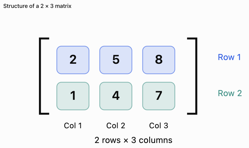
Matrix notation
An element of a matrix can be identified using two subscripts.
For example:
aᵢⱼ
where:
-
i identifies the row.
-
j identifies the column.
For the matrix A above:
a₁₁ = 2
a₁₂ = 5
a₁₃ = 8
a₂₁ = 1
a₂₂ = 4
a₂₃ = 7
Notice that a₂₃ means the element in row 2, column 3.
It does not mean row 3, column 2.
Types of Matrices
Matrices can be classified according to their dimensions and properties.
Row matrix
A matrix containing one row.
Order: 1 × 3
Column matrix
A matrix containing one column.
Order: 3 × 1
Square matrix
A matrix with the same number of rows and columns.
Order: 2 × 2
Zero matrix
A matrix in which every element is zero.
Identity matrix
A square matrix with 1 along the main diagonal and 0 everywhere else.
For example:
The identity matrix has an important role in matrix multiplication.
For any compatible matrix A:
AI = A and IA = A
The identity matrices used on the two sides may have different orders when A is rectangular.
Adding Matrices
Matrix addition combines corresponding elements from two matrices.
Two matrices can be added only when they have the same dimensions.
For example:
Add corresponding elements:
Therefore:
Visualising matrix addition
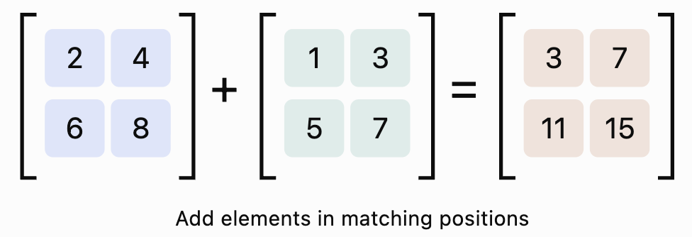
General rule
If A and B are both m × n matrices:
(A + B)ᵢⱼ = aᵢⱼ + bᵢⱼ
The result is also an m × n matrix.
Worked Example 1: Adding 2 × 3 Matrices
Given:
Calculate A + B.
Step 1: Check the dimensions.
Both matrices are 2 × 3.
Addition is possible.
Step 2: Add corresponding elements.
Step 3: Simplify.
Properties of Matrix Addition
Matrix addition has several useful properties.
Commutative property
A + B = B + A
The order of addition does not affect the result.
Associative property
(A + B) + C = A + (B + C)
Matrices can be grouped differently when adding three or more matrices.
Additive identity
A + O = A
Adding a zero matrix of the same dimensions does not change a matrix.
Additive inverse
For every matrix A, there is a matrix −A such that:
A + (−A) = O
The additive inverse is formed by changing the sign of every element.
For example:
Then:
Subtracting Matrices
Matrix subtraction follows the same dimensional rule as addition.
Two matrices can be subtracted only if they have the same dimensions.
Subtract corresponding elements.
Worked Example 2: Matrix Subtraction
Given:
Calculate A − B.
Therefore:
Subtraction as addition of the inverse
Matrix subtraction can also be written as:
A − B = A + (−B)
This relationship is useful when simplifying matrix expressions.
Important distinction
Matrix subtraction is generally not commutative.
A − B ≠ B − A
In fact:
B − A = −(A − B)
Scalar Multiplication
A scalar is a single number.
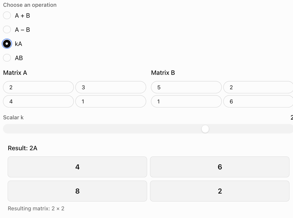
Scalar multiplication means multiplying every element of a matrix by the same number.
For example:
Calculate 3A.
Therefore:
Scalar multiplication does not change the dimensions of the matrix.
Worked Example 3: Multiplying by a Negative Scalar
Given:
Calculate −2B.
Therefore:
Notice that multiplying a negative element by a negative scalar produces a positive result.
Properties of Scalar Multiplication
For scalars k and m and compatible matrices A and B:
Distributive property over matrix addition
k(A + B) = kA + kB
Distributive property over scalar addition
(k + m)A = kA + mA
Associative property
k(mA) = (km)A
Multiplicative identity
1A = A
Multiplication by zero
0A = O
These properties allow matrix expressions to be simplified algebraically.
Worked Example 4: Combining Matrix Operations
Given:
Calculate:
2A − 3B
First:
Next:
Subtract:
Therefore:
Multiplying Matrices
Matrix multiplication is different from matrix addition and scalar multiplication.
We do not simply multiply corresponding elements.
Instead, each element of the resulting matrix is calculated using a row from the first matrix and a column from the second matrix.
The compatibility rule
Suppose:
A has dimensions m × n.
B has dimensions n × p.
Then the product AB is possible, and the result has dimensions:
m × p
The inner dimensions must match.
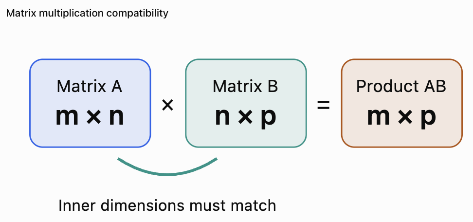
|
Matrix A |
Matrix B |
Is AB possible? |
Result |
|---|---|---|---|
|
2 × 3 |
3 × 4 |
Yes |
2 × 4 |
|
3 × 2 |
2 × 5 |
Yes |
3 × 5 |
|
2 × 2 |
2 × 2 |
Yes |
2 × 2 |
|
3 × 4 |
3 × 2 |
No |
Undefined |
|
1 × 3 |
3 × 1 |
Yes |
1 × 1 |
|
3 × 1 |
1 × 3 |
Yes |
3 × 3 |
The outer dimensions determine the size of the result.
How Matrix Multiplication Works
Consider:
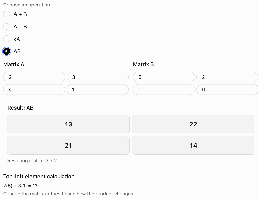
To calculate AB, multiply each row of A by each column of B and add the products.
Finding the first element
Use row 1 of A:
[2, 3]
and column 1 of B:
[5, 1]
Calculate:
2(5) + 3(1) = 13
This becomes the element in row 1, column 1 of AB.
Visualising row-by-column multiplication
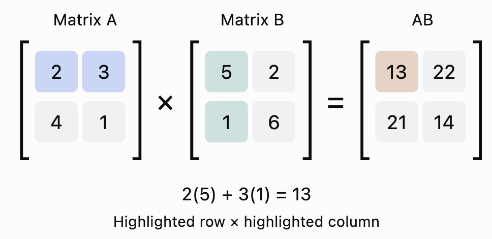
Calculating the complete product
Top-left:
2(5) + 3(1) = 13
Top-right:
2(2) + 3(6) = 22
Bottom-left:
4(5) + 1(1) = 21
Bottom-right:
4(2) + 1(6) = 14
Therefore:
General formula
For compatible matrices A and B:
cᵢⱼ = Σ aᵢₖbₖⱼ
The sum is taken over all matching positions k in the row of A and column of B.
In words:
Multiply corresponding entries from the row and column, then add the products.
Worked Example 5: Multiplying a 2 × 3 Matrix by a 3 × 2 Matrix
Given:
Calculate AB.
Step 1: Check compatibility.
A is 2 × 3.
B is 3 × 2.
The inner dimensions are both 3.
Multiplication is possible.
The result will be 2 × 2.
Step 2: Calculate each element.
Row 1 × Column 1:
1(7) + 2(9) + 3(11)
= 7 + 18 + 33
= 58
Row 1 × Column 2:
1(8) + 2(10) + 3(12)
= 8 + 20 + 36
= 64
Row 2 × Column 1:
4(7) + 5(9) + 6(11)
= 28 + 45 + 66
= 139
Row 2 × Column 2:
4(8) + 5(10) + 6(12)
= 32 + 50 + 72
= 154
Step 3: Write the result.
Worked Example 6: Multiplying a Matrix by a Column Vector
Given:
and:
Calculate Ax.
Step 1: Check dimensions.
A is 2 × 2.
x is 2 × 1.
Multiplication is possible.
The result will be 2 × 1.
Step 2: Multiply rows by the column.
First element:
2(5) + 3(2) = 16
Second element:
1(5) + 4(2) = 13
Therefore:
This type of multiplication is especially important in linear algebra, coordinate transformations, and systems of equations.
Why Matrix Multiplication Is Not Usually Commutative
Ordinary multiplication is commutative:
3 × 5 = 5 × 3
However, matrix multiplication generally is not.
AB ≠ BA
Consider:
Calculate AB:
Now calculate BA:
Therefore:
AB ≠ BA
The order matters because multiplying rows by columns produces different combinations of elements.
Sometimes AB is defined while BA is not.
For example:
A: 2 × 3
B: 3 × 4
AB is possible and has dimensions 2 × 4.
BA is not possible because its inner dimensions would be 4 and 2.
Properties of Matrix Multiplication
For compatible matrices:
Associative property
(AB)C = A(BC)
The grouping of multiplication can change without changing the result.
Distributive property
A(B + C) = AB + AC
and:
(A + B)C = AC + BC
provided the operations are defined.
Identity property
AI = A
and:
IA = A
using identity matrices of suitable dimensions.
Scalar compatibility
k(AB) = (kA)B = A(kB)
Noncommutative property
In general:
AB ≠ BA
Zero product property
Unlike ordinary real numbers, it is possible for two nonzero matrices to have a zero product.
For example:
Both matrices are nonzero, but:
AB = O
This is an important difference between ordinary arithmetic and matrix algebra.
Determining Whether Operations Are Possible
Before performing any matrix operation, always check the dimensions.
Addition and subtraction
The matrices must have identical dimensions.
For example:
2 × 3 + 2 × 3 is possible.
2 × 3 + 3 × 2 is not possible.
Scalar multiplication
A scalar can multiply a matrix of any dimensions.
For example:
5A is possible for any matrix A.
Matrix multiplication
The number of columns in the first matrix must equal the number of rows in the second matrix.
For example:
(2 × 4)(4 × 3) is possible.
The result is 2 × 3.
However:
(2 × 4)(2 × 3) is not possible.
Quick compatibility guide
|
Operation |
Requirement |
Result |
|---|---|---|
|
A + B |
Same dimensions |
Same dimensions |
|
A − B |
Same dimensions |
Same dimensions |
|
kA |
Any matrix A |
Same dimensions as A |
|
AB |
Columns of A = rows of B |
Rows of A × columns of B |
|
BA |
Columns of B = rows of A |
Rows of B × columns of A |
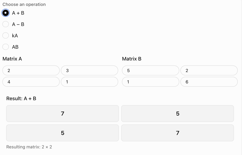
Interactive Matrix Operations Explorer
Explore how addition, subtraction, scalar multiplication, and matrix multiplication work.
Matrix Operations in Real-World Problems
Application 1: Combining Sales Data
Two shops sell three products.
Their weekly sales are represented by:
and:
Rows represent shops.
Columns represent products.
The total sales are:
This provides a compact summary of sales across both weeks.
Application 2: Increasing Production
A factory produces:
If production doubles, the new production matrix is:
Scalar multiplication allows every quantity to be adjusted simultaneously.
Application 3: Calculating Revenue
A shop sells three products.
Quantities sold in two stores are:
The prices of the three products are:
The revenue for each store is calculated using:
R = Qp
Therefore:
-
Store 1 earns $170.
-
Store 2 earns $176.
Matrix multiplication allows the quantities and prices to be combined efficiently.
Matrices and Geometric Transformations
Matrices can describe transformations of points in a coordinate plane.
A point can be represented by a column vector:
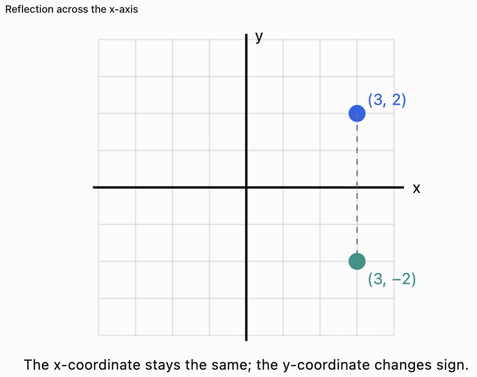
Reflection in the x-axis
The transformation matrix is:
For the point (3, 2):
Calculate:
The point (3, 2) is reflected to (3, −2).
Other transformation matrices can represent:
-
Rotations
-
Reflections
-
Stretches
-
Compressions
-
Shears
These transformations are widely used in computer graphics, animation, robotics, and engineering.
Solving Matrix Equations
Matrix operations can also be used to solve equations involving unknown matrices.
Worked Example 7: Finding an Unknown Matrix
Suppose:
X + A = B
where:
Find X.
Subtract A from both sides:
X = B − A
Therefore:
Worked Example 8: Solving a Matrix Equation with Scalars
Suppose:
2X + A = B
where:
Subtract A:
2X = B − A
Divide every element by 2:
This is equivalent to multiplying the matrix by the scalar 1/2.
Common Mistakes
Mistake 1: Adding matrices with different dimensions
Matrices must have identical dimensions for addition or subtraction.
Mistake 2: Confusing rows and columns
A 2 × 3 matrix has two rows and three columns.
Mistake 3: Forgetting to multiply every element by a scalar
Scalar multiplication affects every element.
Mistake 4: Multiplying corresponding elements during matrix multiplication
Matrix multiplication uses row-by-column products and sums.
Mistake 5: Ignoring the inner dimensions
AB is possible only when the columns of A equal the rows of B.
Mistake 6: Assuming AB = BA
Matrix multiplication is generally not commutative.
Mistake 7: Predicting the wrong result dimensions
The result of an m × n matrix multiplied by an n × p matrix is m × p.
Mistake 8: Making sign errors
Negative elements require careful handling.
Mistake 9: Reversing the order of multiplication
AB and BA may produce different results or one may be undefined.
Mistake 10: Forgetting to interpret the result
In applications, matrix elements represent real quantities such as prices, distances, or measurements.
Key Terms
-
Matrix: Rectangular arrangement of elements in rows and columns.
-
Element: Individual entry in a matrix.
-
Row: Horizontal arrangement of elements.
-
Column: Vertical arrangement of elements.
-
Order: Dimensions of a matrix, written as rows × columns.
-
Row Matrix: Matrix containing one row.
-
Column Matrix: Matrix containing one column.
-
Square Matrix: Matrix with equal numbers of rows and columns.
-
Zero Matrix: Matrix in which every element is zero.
-
Identity Matrix: Square matrix with 1 on the main diagonal and 0 elsewhere.
-
Scalar: Single number used to multiply a matrix.
-
Matrix Addition: Operation combining corresponding elements of matrices with identical dimensions.
-
Matrix Subtraction: Operation subtracting corresponding elements.
-
Scalar Multiplication: Multiplication of every matrix element by a scalar.
-
Matrix Multiplication: Operation combining rows and columns through products and sums.
-
Compatible Matrices: Matrices whose dimensions allow a particular operation.
-
Matrix Product: Result of multiplying compatible matrices.
-
Commutative Property: Property stating that changing the order of an operation does not change the result.
-
Associative Property: Property allowing the grouping of operations to change.
-
Distributive Property: Property relating multiplication to addition.
-
Additive Inverse: Matrix that produces the zero matrix when added to the original.
-
Transformation Matrix: Matrix representing a geometric transformation.
-
Column Vector: Matrix consisting of one column.
-
Matrix Equation: Equation containing one or more matrices.
-
Linear Algebra: Branch of mathematics involving vectors, matrices, and linear relationships.
Key Takeaways
-
Matrices organise information into rows and columns.
-
Matrix dimensions are written as rows × columns.
-
Matrices can be added or subtracted only when they have identical dimensions.
-
Addition and subtraction are performed element by element.
-
Scalar multiplication multiplies every element by the same number.
-
Matrix multiplication requires compatible inner dimensions.
-
The result of multiplying an m × n matrix by an n × p matrix has dimensions m × p.
-
Matrix multiplication uses row-by-column calculations.
-
Matrix multiplication is generally not commutative.
-
Addition and scalar multiplication follow useful algebraic properties.
-
Identity matrices play a role similar to the number 1 in multiplication.
-
Matrices can represent data, transformations, and systems of equations.
-
Matrix operations are useful in finance, science, engineering, and computer graphics.
-
Checking dimensions before calculating helps prevent errors.
Check Your Understanding
Questions
Question 1: Matrix Dimensions
Determine the dimensions of:
Question 2: Matrix Addition
Calculate:
Question 3: Matrix Subtraction
Calculate:
Question 4: Scalar Multiplication
Calculate:
Question 5: Negative Scalar
Calculate:
Question 6: Compatibility
Determine whether the product AB is possible if:
A is 3 × 4.
B is 4 × 2.
State the dimensions of the result.
Question 7: Incompatible Matrices
Explain why a 2 × 3 matrix cannot be multiplied on the right by a 4 × 2 matrix.
Question 8: Matrix Multiplication
Calculate:
Question 9: Matrix and Column Vector
Calculate:
Question 10: Combined Operations
Given:
Calculate 2A + B.
Question 11: Matrix Equations
Solve:
X + A = B
where:
Question 12: Noncommutative Multiplication
Explain why AB is not always equal to BA.
Question 13: Revenue Calculation
A shop sells two products.
The quantities sold are:
The prices are:
Calculate Qp and interpret the result.
Question 14: Geometric Transformation
Use the matrix:
to transform the point (4, 3).
Question 15: Integrated Matrix Challenge
Given:
Calculate:
a) A + B
b) A − B
c) 3A
d) AB
e) BA
f) Explain whether AB = BA.
Fully Worked Answers
Answer 1: Matrix Dimensions
The matrix has two rows and three columns.
Answer: 2 × 3
Answer 2: Matrix Addition
Answer 3: Matrix Subtraction
Answer 4: Scalar Multiplication
Answer 5: Negative Scalar
Answer 6: Compatibility
A is 3 × 4.
B is 4 × 2.
The inner dimensions are both 4.
Multiplication is possible.
Result: 3 × 2
Answer 7: Incompatible Matrices
A is 2 × 3.
B is 4 × 2.
The inner dimensions are 3 and 4.
They do not match.
Therefore, AB is undefined.
Answer 8: Matrix Multiplication
Top-left:
1(5) + 2(7) = 19
Top-right:
1(6) + 2(8) = 22
Bottom-left:
3(5) + 4(7) = 43
Bottom-right:
3(6) + 4(8) = 50
Answer 9: Matrix and Column Vector
First element:
2(5) + 1(2) = 12
Second element:
4(5) + 3(2) = 26
Answer 10: Combined Operations
First:
Add B:
Answer 11: Matrix Equations
Given:
X + A = B
Subtract A:
X = B − A
Answer 12: Noncommutative Multiplication
Matrix multiplication uses rows from the first matrix and columns from the second matrix.
Reversing the order changes which rows and columns are combined.
Therefore, AB and BA generally produce different results.
Sometimes one product is possible while the other is undefined.
Answer 13: Revenue Calculation
First store:
10(4) + 20(6)
= 40 + 120
= 160
Second store:
15(4) + 12(6)
= 60 + 72
= 132
The first store earns $160.
The second store earns $132.
Answer 14: Geometric Transformation
Given:
and:
Calculate:
Answer: (−4, 3)
The transformation is a reflection in the y-axis.
Answer 15: Integrated Matrix Challenge
Given:
Part a: A + B
Part b: A − B
Part c: 3A
Part d: AB
Top-left:
2(1) + 1(2) = 4
Top-right:
2(5) + 1(3) = 13
Bottom-left:
3(1) + 4(2) = 11
Bottom-right:
3(5) + 4(3) = 27
Part e: BA
Top-left:
1(2) + 5(3) = 17
Top-right:
1(1) + 5(4) = 21
Bottom-left:
2(2) + 3(3) = 13
Bottom-right:
2(1) + 3(4) = 14
Part f: Compare AB and BA
The matrices are different.
Therefore:
AB ≠ BA
This demonstrates that matrix multiplication is not generally commutative.
Final Reflection
Matrix operations extend familiar arithmetic ideas into a powerful system for working with organised numerical information.
Addition and subtraction allow us to combine or compare datasets. Scalar multiplication changes every element by the same factor. Matrix multiplication creates new relationships by combining rows and columns.
These operations are not arbitrary rules. They provide the mathematical foundation for many important applications, including computer graphics, engineering, scientific modeling, economics, and systems of equations.
One of the most important skills is recognising when an operation is possible. Checking matrix dimensions before calculating prevents many common errors.
The central idea is that matrices allow us to organise and manipulate multiple related quantities efficiently, while the rules of matrix operations ensure that the calculations remain mathematically meaningful.