Applications and Connections
2. Scientific Applications
Learning outcomes
- I can model radioactive decay.
- I can analyse chemical concentration scales.
- I can model biological growth.
- I can interpret exponential relationships in science.
- I can solve authentic scientific problems.
Introduction
Many scientific processes involve quantities that change over time or vary across enormous ranges of values.
A radioactive substance gradually loses unstable nuclei. Bacterial populations can increase rapidly when conditions are favourable. Chemical concentrations can differ by factors of thousands or millions, while the acidity of a solution may change dramatically with only a small change in pH.
These processes may appear unrelated, but they share important mathematical foundations: exponential functions, logarithms, rates of change, and mathematical modelling.
Consider these questions:
-
How much radioactive material remains after several half-lives?
-
How can we calculate the age of a sample using radioactive decay?
-
Why does a solution with pH 3 have ten times the hydrogen ion activity of a solution with pH 4?
-
How quickly can a bacterial population double?
-
Why do some biological populations grow exponentially at first but eventually slow down?
-
How can we use scientific measurements to determine unknown growth or decay constants?
In this lesson, we will explore how exponential and logarithmic models describe radioactive decay, chemical concentration scales, biological growth, and other scientific phenomena.
We will also investigate the assumptions and limitations of these models, because a useful scientific model must do more than produce a numerical answer: it must represent the physical, chemical, or biological situation meaningfully.
Exponential Relationships in Science
An exponential relationship occurs when a quantity changes at a rate proportional to its current value.
A common model is:
Q(t) = Q₀eᵏᵗ
Where:
-
Q(t) = quantity at time t.
-
Q₀ = initial quantity.
-
e ≈ 2.71828.
-
k = signed continuous growth or decay constant.
-
t = elapsed time.
If k > 0, the quantity increases exponentially.
If k < 0, the quantity decreases exponentially.
Why exponential relationships occur
Suppose a bacterial population grows at a rate proportional to the number of bacteria already present.
A larger population contains more organisms capable of reproduction, so the total rate of growth increases.
Similarly, in radioactive decay, a larger sample contains more unstable nuclei available to decay, so the expected number of decays per unit time is greater.
The mathematical relationship is:
dQ/dt = kQ
This states that the instantaneous rate of change is proportional to the current quantity.
Solving this differential equation gives the exponential model.
Exponential growth versus exponential decay
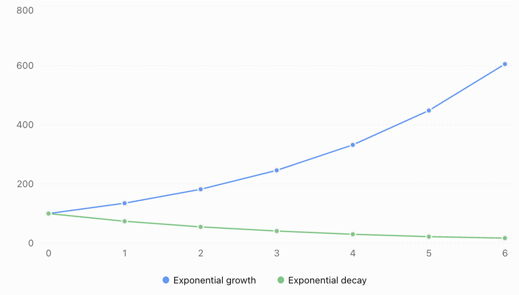
Both curves are exponential, but their behaviour is different.
For exponential growth, equal time intervals produce the same multiplication factor greater than one.
For exponential decay, equal time intervals produce the same multiplication factor between zero and one.
Radioactive Decay
Radioactive decay is the spontaneous transformation of an unstable atomic nucleus into a different nuclear state or another nucleus, often accompanied by the emission of radiation.
Examples of radioactive isotopes include carbon-14, iodine-131, uranium-238, and cobalt-60.
The decay of an individual nucleus is unpredictable. However, when a sample contains a very large number of radioactive nuclei, the expected number remaining follows a predictable exponential relationship.
The radioactive decay equation
Radioactive decay is commonly written as:
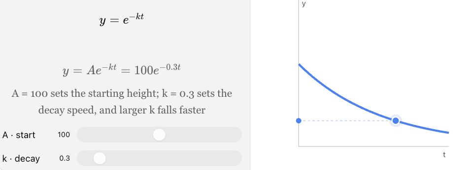
N(t) = N₀e⁻λᵗ
Where:
-
N(t) = expected number of undecayed radioactive nuclei at time t.
-
N₀ = initial number of radioactive nuclei.
-
λ = positive decay constant.
-
t = elapsed time.
The decay constant has units of inverse time, such as s⁻¹, day⁻¹, or year⁻¹.
A larger decay constant means faster radioactive decay.
Visualising exponential decay
How the decay constant changes the curve
Half-Life
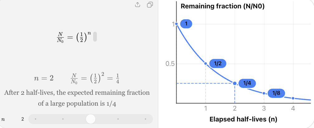
The half-life of a radioactive isotope is the time required for the expected number of undecayed nuclei in a large sample to decrease to half its original value.
After one half-life, 50% remains.
After two half-lives, 25% remains.
After three half-lives, 12.5% remains.
After four half-lives, 6.25% remains.
|
Number of half-lives |
Fraction remaining |
Percentage remaining |
|---|---|---|
|
0 |
1 |
100% |
|
1 |
1/2 |
50% |
|
2 |
1/4 |
25% |
|
3 |
1/8 |
12.5% |
|
4 |
1/16 |
6.25% |
|
5 |
1/32 |
3.125% |
The half-life formula
Half-life and decay constant are related by:
t½ = ln(2)/λ
Equivalently:
λ = ln(2)/t½
These equations allow us to calculate one quantity when the other is known.
Worked Example 1: Radioactive Material Remaining
A radioactive sample initially contains 160 g of a particular isotope.
Its half-life is 8 days.
Calculate the amount remaining after 24 days.
Step 1: Calculate the number of half-lives.
Number of half-lives = 24/8
Number of half-lives = 3
Step 2: Apply the half-life relationship.
Remaining mass = 160 × (1/2)³
Remaining mass = 160 × 1/8
Remaining mass = 20 g
After 24 days, the expected remaining mass of the original isotope is 20 g.
Worked Example 2: Finding the Decay Constant
An isotope has a half-life of 12 hours.
Calculate its decay constant.
Use:
λ = ln(2)/t½
Substitute:
λ = ln(2)/12
λ = 0.693147/12
λ ≈ 0.05776 h⁻¹
The exponential decay model is:
N(t) = N₀e⁻⁰·⁰⁵⁷⁷⁶ᵗ
where t is measured in hours.
Worked Example 3: Finding the Time Required for Decay
A radioactive sample follows:
M(t) = 500e⁻⁰·⁰⁸ᵗ
where M is measured in grams and t in years.
How long will it take for the sample to decrease to 100 g of the original isotope?
Step 1: Substitute the target mass.
100 = 500e⁻⁰·⁰⁸ᵗ
Step 2: Divide by 500.
0.2 = e⁻⁰·⁰⁸ᵗ
Step 3: Take natural logarithms.
ln(0.2) = −0.08t
Step 4: Solve.
t = ln(0.2)/(−0.08)
t ≈ −1.609438/(−0.08)
t ≈ 20.12 years
The sample reaches 100 g after approximately 20.12 years.
Radioactive Activity
The activity of a radioactive sample is the number of nuclear decays per unit time.
The SI unit of activity is the becquerel (Bq).
1 Bq = 1 decay per second
For a large sample:
A = λN
Where:
-
A = activity in Bq.
-
λ = decay constant in s⁻¹.
-
N = number of undecayed radioactive nuclei.
Because the number of radioactive nuclei decreases exponentially, activity also decreases exponentially:
A(t) = A₀e⁻λᵗ
Worked Example 4: Radioactive Activity
A sample initially has an activity of 800 Bq.
Its half-life is 5 hours.
Calculate its expected activity after 15 hours.
Number of half-lives:
15/5 = 3
Activity remaining:
A = 800 × (1/2)³
A = 800/8
A = 100 Bq
The expected activity after 15 hours is 100 Bq.
The activity and the number of undecayed nuclei have the same half-life.
Radiometric Dating
Radioactive decay can be used to estimate the age of certain materials.
Radiometric dating relies on measuring radioactive isotopes and interpreting how their quantities have changed over time.
One example is carbon-14 dating.
Carbon-14 is a radioactive isotope that is incorporated into living organisms through the carbon cycle.
After an organism dies, it generally stops exchanging carbon with its environment, and the carbon-14 already present continues to decay.
The half-life of carbon-14 is approximately 5,730 years.
Worked Example 5: Carbon-14 Dating
An archaeological sample contains 25% of the carbon-14 activity expected for a comparable modern sample.
Assume the sample has remained a closed system and the initial activity is appropriately estimated.
Estimate its age.
Step 1: Determine the remaining fraction.
25% = 0.25 = 1/4
Step 2: Express the fraction as powers of one-half.
1/4 = (1/2)²
Therefore, two half-lives have elapsed.
Step 3: Calculate the age.
Age = 2 × 5730
Estimated age = 11,460 years
In real radiocarbon dating, measured ages require calibration and may be affected by contamination, reservoir effects, and uncertainty in the initial carbon-14 activity.
The calculation above demonstrates the mathematical principle.
Interpreting Radioactive Decay Critically
Radioactive decay models are powerful because the decay constant is characteristic of a particular nuclear state under ordinary conditions.
However, several limitations must be recognised.
-
Radioactive decay is probabilistic at the level of individual nuclei.
-
The exponential law describes expected behaviour for large populations of nuclei.
-
Measuring instruments have uncertainties and background radiation.
-
Samples may contain mixtures of isotopes.
-
Radiometric dating requires assumptions about the original material and possible contamination.
The mathematics is reliable within the model, but scientific conclusions also depend on measurement quality and appropriate interpretation.
Chemical Concentration Scales
Chemists frequently work with extremely small or extremely large concentration ratios.
Logarithmic scales are useful because they compress large numerical ranges into manageable values.
One important example is the pH scale.
Understanding pH
pH is a logarithmic measure related to hydrogen ion activity in a solution.
The thermodynamic definition is:
pH = −log₁₀(aH⁺)
where aH⁺ is the dimensionless activity of hydrogen ions.
For many introductory calculations involving sufficiently dilute aqueous solutions, activity is approximated using molar concentration:
pH ≈ −log₁₀([H⁺]/(1 mol/L))
It is common in school-level chemistry to write the approximation as:
pH = −log₁₀[H⁺]
with [H⁺] understood to be the numerical concentration in mol/L under the dilute-solution approximation.
Why is pH logarithmic?
Hydrogen ion concentrations may vary by many orders of magnitude.
A logarithmic scale makes these differences easier to compare.
For example:
-
pH 2 corresponds approximately to [H⁺] = 10⁻² mol/L.
-
pH 3 corresponds approximately to [H⁺] = 10⁻³ mol/L.
-
pH 4 corresponds approximately to [H⁺] = 10⁻⁴ mol/L.
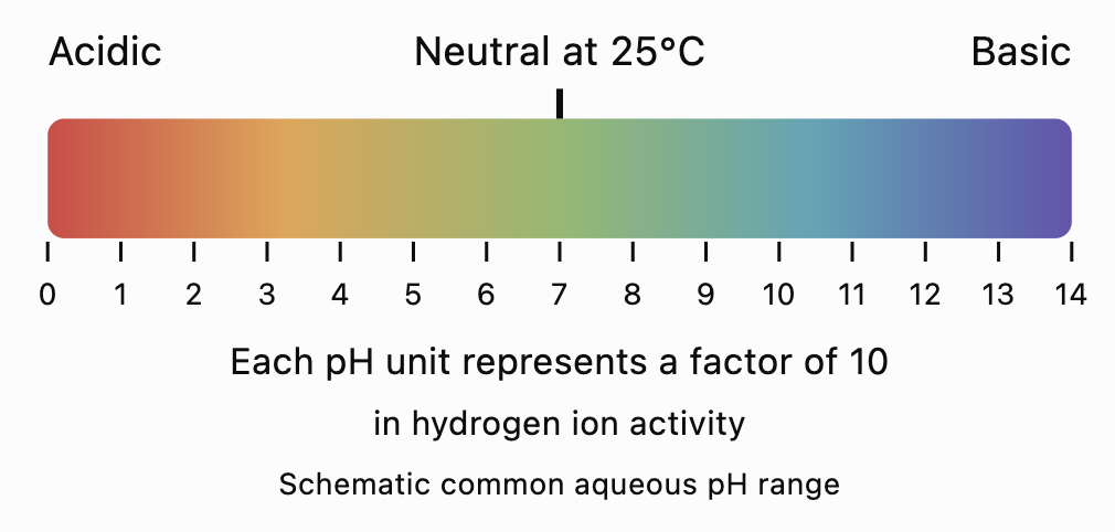
A decrease of one pH unit corresponds to a tenfold increase in hydrogen ion activity.
Understanding the pH scale
Worked Example 6: Calculating pH
A dilute aqueous solution has a hydrogen ion concentration of:
[H⁺] = 1 × 10⁻⁴ mol/L
Calculate its approximate pH.
Use:
pH ≈ −log₁₀(10⁻⁴)
Since log₁₀(10⁻⁴) = −4:
pH ≈ −(−4)
pH ≈ 4
The solution is acidic.
Worked Example 7: Finding Hydrogen Ion Concentration
A dilute aqueous solution has pH = 3.5.
Calculate its approximate hydrogen ion concentration.
Start with:
pH ≈ −log₁₀([H⁺])
Rearrange:
[H⁺] ≈ 10⁻ᵖᴴ mol/L
Substitute:
[H⁺] ≈ 10⁻³·⁵
[H⁺] ≈ 3.16 × 10⁻⁴ mol/L
Worked Example 8: Comparing Acidity
Solution A has pH 2.
Solution B has pH 5.
How many times greater is the hydrogen ion activity in Solution A?
The difference in pH is:
5 − 2 = 3
Each pH unit represents a factor of 10.
Therefore:
Ratio = 10³
Ratio = 1,000
Solution A has 1,000 times the hydrogen ion activity of Solution B.
This does not necessarily mean it contains 1,000 times the total amount of acid, because acid concentration, dissociation, and buffering also matter.
The pOH Scale
Another logarithmic chemical scale is pOH.
For dilute aqueous solutions:
pOH ≈ −log₁₀([OH⁻]/(1 mol/L))
At 25°C, for dilute aqueous solutions:
pH + pOH ≈ 14
Worked Example 9: Calculating pOH
A solution has pH = 9.2 at 25°C.
Calculate pOH.
pOH ≈ 14 − 9.2
pOH ≈ 4.8
The solution is basic.
At temperatures other than 25°C, the relationship changes because the ion product of water changes.
Other Logarithmic Scales in Science
Logarithms are useful wherever quantities span very large ranges.
Sound intensity level
Sound intensity level is measured in decibels.
β = 10log₁₀(I/I₀)
Where:
-
β = sound intensity level in decibels.
-
I = sound intensity.
-
I₀ = reference intensity.
For sound intensity in air, a commonly used reference is:
I₀ = 10⁻¹² W/m²
Worked Example 10: Comparing Sound Intensities
Two sounds have intensity levels of 60 dB and 80 dB.
Find the ratio of their intensities.
Difference:
80 − 60 = 20 dB
Using:
20 = 10log₁₀(I₂/I₁)
Divide by 10:
2 = log₁₀(I₂/I₁)
Convert to exponential form:
I₂/I₁ = 10²
I₂/I₁ = 100
The 80 dB sound has 100 times the physical intensity of the 60 dB sound, assuming the same reference intensity.
This does not mean it is perceived as 100 times as loud.
Why logarithmic scales are useful
A logarithmic scale converts multiplication into addition.
For example:
log₁₀(1000) = 3
log₁₀(10000) = 4
A tenfold increase produces an increase of one logarithmic unit.
This makes logarithmic scales particularly useful for quantities varying across many orders of magnitude.
Biological Growth Models
Living organisms reproduce, develop, compete for resources, and respond to their environment. Mathematical models help scientists investigate these processes.
Two particularly important biological models are exponential growth and logistic growth.
Exponential Population Growth
Exponential growth occurs when the instantaneous rate of population increase is proportional to the current population.
The model is:
P(t) = P₀eʳᵗ
Where:
-
P(t) = population at time t.
-
P₀ = initial population.
-
r = positive continuous growth constant.
-
t = time.
This model assumes that the relative growth rate remains constant.
Worked Example 11: Bacterial Growth
A bacterial culture initially contains 500 bacteria.
Under ideal laboratory conditions, the population grows continuously at a rate of 0.4 per hour.
Calculate the expected population after six hours.
Step 1: Write the model.
P(t) = 500e⁰·⁴ᵗ
Step 2: Substitute t = 6.
P(6) = 500e^(0.4 × 6)
P(6) = 500e²·⁴
Step 3: Evaluate.
e²·⁴ ≈ 11.02318
P(6) ≈ 500 × 11.02318
P(6) ≈ 5,512 bacteria
The model predicts approximately 5,512 bacteria after six hours.
This prediction assumes that nutrients, space, temperature, and other conditions remain suitable for continued growth.
Doubling Time in Biology
Doubling time describes how long a growing population takes to become twice its initial size.
For continuous exponential growth:
tᵈ = ln(2)/r
Where r > 0.
Worked Example 12: Calculating Bacterial Doubling Time
A bacterial population grows continuously at a rate of 0.35 per hour.
Calculate its doubling time.
tᵈ = ln(2)/0.35
tᵈ = 0.693147/0.35
tᵈ ≈ 1.98 hours
The population doubles approximately every 1.98 hours.
Interpreting the result
A constant doubling time means that the population multiplies by the same factor over equal time intervals.
However, the absolute increase becomes larger as the population grows.
For example, doubling from 100 to 200 adds 100 organisms.
Doubling from 10,000 to 20,000 adds 10,000 organisms.
The proportional change is the same, but the numerical increase is different.
Logistic Growth in Biology
Exponential growth cannot usually continue indefinitely in a limited environment.
As a population increases, resources become scarcer and competition becomes more significant.
A logistic model accounts for these limitations.
The standard logistic function is:
P(t) = K/(1 + Ae⁻ʳᵗ)
Where:
-
K = carrying capacity.
-
A = constant determined by the initial population.
-
r = intrinsic growth parameter.
-
t = time.
For an initial population P₀:
A = (K − P₀)/P₀
Comparing exponential and logistic growth
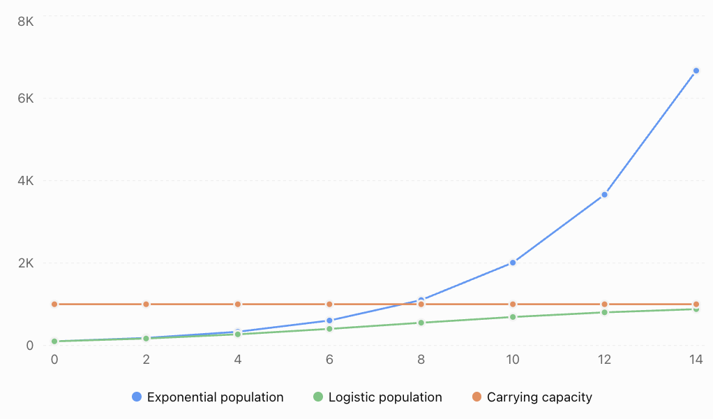
Both models begin with 100 organisms and use a growth parameter of 0.3 per hour. The logistic model includes a carrying capacity of 1,000.
The exponential model predicts continued rapid growth.
The logistic model predicts that growth slows as the population approaches carrying capacity.
Worked Example 13: Logistic Bacterial Growth
A bacterial culture begins with 200 organisms.
The carrying capacity of its environment is 5,000 organisms, and the intrinsic growth parameter is 0.5 per hour.
Calculate the expected population after eight hours.
Step 1: Calculate A.
A = (K − P₀)/P₀
A = (5000 − 200)/200
A = 4800/200
A = 24
Step 2: Write the model.
P(t) = 5000/(1 + 24e⁻⁰·⁵ᵗ)
Step 3: Substitute t = 8.
P(8) = 5000/(1 + 24e⁻⁴)
Step 4: Evaluate.
e⁻⁴ ≈ 0.0183156
P(8) ≈ 5000/[1 + 24(0.0183156)]
P(8) ≈ 5000/1.439575
P(8) ≈ 3,473 bacteria
The population is predicted to reach approximately 3,473 organisms after eight hours.
The model predicts that the population will gradually approach 5,000 rather than grow without limit.
Interpreting Carrying Capacity
Carrying capacity represents the population size that an environment can sustain under the conditions assumed by the model.
It may depend on:
-
Food and nutrient availability.
-
Water supply.
-
Available space.
-
Competition.
-
Waste accumulation.
-
Predation and disease.
-
Temperature and other environmental conditions.
Carrying capacity is not necessarily permanent.
A change in environmental conditions may increase or decrease the number of organisms that can be supported.
Other Scientific Exponential Applications
Exponential functions are not limited to radioactive decay and biological growth.
They also describe several important processes in chemistry, physics, and environmental science.
First-Order Chemical Reactions
In a first-order chemical reaction, the rate of disappearance of a reactant is proportional to its concentration.
For a reactant A:
d[A]/dt = −k[A]
The integrated rate law is:
A = [A]₀e⁻ᵏᵗ
Where:
-
A = reactant concentration at time t.
-
[A]₀ = initial concentration.
-
k = first-order rate constant.
-
t = time.
The mathematical form is the same as radioactive decay.
However, the underlying physical processes are different.
Radioactive decay involves nuclear transformations, while chemical reactions involve rearrangements of atoms and chemical bonds.
Worked Example 14: First-Order Reaction
A reactant has an initial concentration of 0.80 mol/L.
Its concentration follows first-order kinetics with k = 0.15 min⁻¹.
Calculate the concentration after 10 minutes.
A = 0.80e⁻⁰·¹⁵ᵗ
A = 0.80e⁻¹·⁵
Since e⁻¹·⁵ ≈ 0.223130:
A ≈ 0.80 × 0.223130
A ≈ 0.179 mol/L
The reactant concentration decreases to approximately 0.179 mol/L.
Newton's Law of Cooling
The rate at which an object cools is often approximately proportional to the temperature difference between the object and its surroundings.
For constant ambient temperature:
T(t) = Tₐ + (T₀ − Tₐ)e⁻ᵏᵗ
Where:
-
T(t) = object temperature at time t.
-
Tₐ = ambient temperature.
-
T₀ = initial object temperature.
-
k = positive cooling constant.
The temperature difference, T − Tₐ, decreases exponentially.
Worked Example 15: Cooling Coffee
A cup of coffee begins at 85°C in a room at 25°C.
The cooling constant is 0.08 min⁻¹.
Calculate the coffee's temperature after 15 minutes.
T(t) = 25 + (85 − 25)e⁻⁰·⁰⁸ᵗ
T(15) = 25 + 60e⁻¹·²
Since e⁻¹·² ≈ 0.301194:
T(15) ≈ 25 + 60(0.301194)
T(15) ≈ 25 + 18.0716
T(15) ≈ 43.07°C
The coffee is predicted to cool to approximately 43.1°C.
It approaches room temperature rather than approaching 0°C.
Light Absorption and Concentration
Another important scientific relationship is the Beer–Lambert law.
For a suitable solution:
A = εlc
Where:
-
A = absorbance.
-
ε = molar absorption coefficient.
-
l = optical path length.
-
c = concentration.
Absorbance is defined by:
A = log₁₀(I₀/I)
Where:
-
I₀ = incident light intensity.
-
I = transmitted light intensity.
Therefore:
I = I₀ × 10⁻ᴬ
Combining the relationships:
I = I₀ × 10⁻εˡᶜ
This means that transmitted light intensity decreases exponentially with concentration when ε and l are constant.
Worked Example 16: Absorbance
A solution has absorbance A = 0.60.
Calculate the fraction of incident light transmitted.
I/I₀ = 10⁻⁰·⁶⁰
I/I₀ ≈ 0.2512
Transmitted fraction ≈ 0.251
Approximately 25.1% of the incident light is transmitted.
This relationship is widely used in spectrophotometry to investigate chemical concentrations.
Interpreting Exponential Relationships Critically
Exponential models share a common mathematical form, but their parameters must be interpreted in context.
Consider three models:
Radioactive decay
N(t) = 1000e⁻⁰·²ᵗ
Bacterial growth
P(t) = 1000e⁰·²ᵗ
Chemical concentration
C(t) = 0.50e⁻⁰·²ᵗ
Although these equations use the same numerical magnitude for the exponential constant, they describe different quantities.
The meaning of the constant depends on the process and the units of time.
|
Model |
Initial quantity |
Constant |
Interpretation |
|---|---|---|---|
|
Radioactive decay |
1,000 nuclei |
−0.2 |
Expected number decreases |
|
Bacterial growth |
1,000 organisms |
+0.2 |
Population increases |
|
Chemical concentration |
0.50 mol/L |
−0.2 |
Concentration decreases |
A mathematical model must always be accompanied by clearly defined variables and units.
Estimating a Growth or Decay Constant from Data
Suppose a quantity follows:
Q(t) = Q₀eᵏᵗ
Taking natural logarithms gives:
ln[Q(t)/Q₀] = kt
Therefore:
k = ln[Q(t)/Q₀]/t
This formula works for both growth and decay.
For growth, k is positive.
For decay, k is negative.
Worked Example 17: Estimating a Decay Constant
A chemical concentration decreases from 0.60 mol/L to 0.24 mol/L in eight minutes.
Assume first-order decay.
Find the decay constant.
Step 1: Substitute the values.
k = ln(0.24/0.60)/8
k = ln(0.4)/8
Step 2: Evaluate.
ln(0.4) ≈ −0.916291
k ≈ −0.916291/8
k ≈ −0.11454 min⁻¹
The signed exponential constant is −0.11454 min⁻¹.
Equivalently, the positive first-order decay constant is:
λ ≈ 0.11454 min⁻¹
The concentration model becomes:
C(t) = 0.60e⁻⁰·¹¹⁴⁵⁴ᵗ
Using Logarithmic Transformations to Analyse Scientific Data
A useful property of exponential models is that taking logarithms converts them into linear relationships.
Starting with:
Q(t) = Q₀eᵏᵗ
Take natural logarithms:
ln[Q(t)] = ln(Q₀) + kt
This has the form:
y = mx + b
where:
-
y = ln[Q(t)]
-
x = t
-
slope = k
-
intercept = ln(Q₀)
Strictly, logarithms must be taken of dimensionless quantities, so a reference unit is understood when logarithms of measured quantities are used.
Why is this useful?
If experimental data follow an exponential model, plotting the natural logarithm of the measured quantity against time should produce an approximately straight line.
The slope can be used to estimate the growth or decay constant.
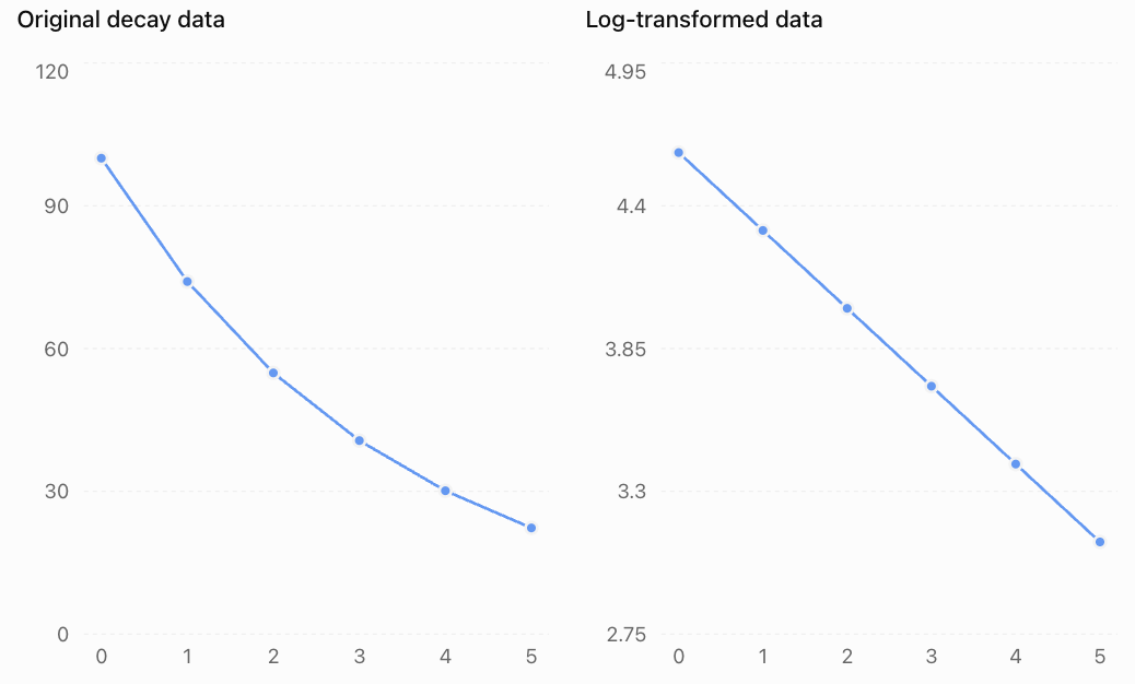
The original quantity decreases exponentially.
The logarithm of the quantity decreases linearly.
In this example, the slope of the transformed graph is approximately −0.3 per unit time.
This suggests a decay constant of 0.3 per unit time.
Important limitation
A straight line on a logarithmic transformation supports an exponential relationship, but it does not prove the underlying process is exponential.
Measurement errors, small datasets, and limited observation ranges can make different models appear similar.
Authentic Scientific Investigation: Evaluating a Bacterial Culture
A scientist grows bacteria in a nutrient solution and records the population.
|
Time (hours) |
Population |
|---|---|
|
0 |
200 |
|
2 |
365 |
|
4 |
665 |
|
6 |
1,211 |
|
8 |
2,207 |
The scientist wants to determine whether exponential growth is an appropriate model.
Step 1: Examine population ratios
For equal two-hour intervals:
365/200 ≈ 1.825
665/365 ≈ 1.822
1211/665 ≈ 1.821
2207/1211 ≈ 1.822
The ratios are approximately constant.
This supports an exponential model.
Step 2: Estimate the growth constant
Using the first and final measurements:
k = ln(2207/200)/8
k = ln(11.035)/8
k ≈ 0.300 per hour
Step 3: Construct the model
P(t) ≈ 200e⁰·³ᵗ
Step 4: Predict the population after 10 hours
P(10) ≈ 200e³
P(10) ≈ 200(20.0855)
P(10) ≈ 4,017 bacteria
Step 5: Evaluate the prediction
The model predicts approximately 4,017 bacteria after 10 hours.
However, the scientist should consider whether nutrients, oxygen, space, or waste accumulation may begin limiting growth.
If the culture approaches environmental carrying capacity, a logistic or other growth model may become more appropriate.
The exponential model is supported by the observed early data, but its long-term reliability has not been established.
Common Mistakes
Mistake 1: Confusing exponential growth and decay
A positive exponential constant represents growth, while a negative constant represents decay.
Correction: Check the sign of the exponent coefficient.
Mistake 2: Subtracting half the original quantity every half-life
After each half-life, half of the amount currently remaining is expected to survive.
Correction: Use repeated multiplication by 1/2.
Mistake 3: Confusing half-life and decay constant
Half-life has units of time, while the decay constant has units of inverse time.
Correction: Use t½ = ln(2)/λ.
Mistake 4: Treating radioactive decay as deterministic for individual atoms
The time at which a particular nucleus decays cannot generally be predicted.
Correction: Interpret exponential decay statistically for large populations of nuclei.
Mistake 5: Treating the pH scale as linear
A difference of one pH unit represents a factor of 10 in hydrogen ion activity, not a fixed additive change.
Correction: Use logarithmic relationships when comparing acidity.
Mistake 6: Confusing logarithms with natural logarithms
The pH scale uses base-10 logarithms, while continuous exponential models commonly use natural logarithms.
Correction: Identify the logarithm base required by the model.
Mistake 7: Ignoring units
A decay constant measured in hours⁻¹ cannot be used directly with time measured in days.
Correction: Convert quantities into consistent units.
Mistake 8: Assuming biological populations grow exponentially forever
Real populations are limited by resources and environmental conditions.
Correction: Evaluate whether a logistic or another resource-limited model is more appropriate.
Mistake 9: Assuming all exponential models describe the same process
Radioactive decay, chemical reactions, and biological growth may have similar equations but different mechanisms.
Correction: Interpret each model using the scientific context.
Mistake 10: Ignoring experimental uncertainty
Measurements contain error, and estimated model parameters may be uncertain.
Correction: Use multiple observations, examine residuals, and communicate limitations.
Key Terms
-
Exponential Growth: Growth in which the instantaneous rate of increase is proportional to the current quantity.
-
Exponential Decay: Decrease in which the instantaneous rate of decrease is proportional to the current quantity.
-
Radioactive Decay: Spontaneous transformation of an unstable atomic nucleus.
-
Half-Life: Time required for the expected remaining radioactive population to decrease by half.
-
Decay Constant: Positive parameter describing the rate of exponential decay.
-
Activity: Number of radioactive decays per unit time.
-
Becquerel (Bq): SI unit of radioactive activity, equal to one decay per second.
-
Radiometric Dating: Estimating the age of materials using radioactive isotope measurements.
-
Carbon-14 Dating: Radiometric dating method using the decay of carbon-14.
-
Hydrogen Ion Activity: Effective thermodynamic measure of hydrogen ions in solution.
-
pH: Logarithmic measure related to hydrogen ion activity.
-
pOH: Logarithmic measure related to hydroxide ion activity.
-
Logarithmic Scale: Scale representing multiplicative changes through additive differences.
-
Decibel: Logarithmic unit used to express ratios, including sound intensity levels.
-
First-Order Reaction: Reaction whose rate is proportional to the concentration of a particular reactant.
-
Rate Constant: Parameter relating a reaction rate to reactant concentrations.
-
Biological Growth: Increase in a biological population or another biological quantity.
-
Doubling Time: Time required for an exponentially growing quantity to double.
-
Logistic Growth: Growth that slows as a population approaches carrying capacity.
-
Carrying Capacity: Population size an environment can sustain under the assumed conditions.
-
Newton's Law of Cooling: Model relating the rate of temperature change to the difference between an object's temperature and its surroundings.
-
Beer–Lambert Law: Relationship connecting absorbance, optical path length, and concentration.
-
Logarithmic Transformation: Applying logarithms to data to simplify or investigate mathematical relationships.
-
Scientific Model: Mathematical or conceptual representation of a scientific process.
-
Model Limitation: A condition restricting the accuracy or applicability of a model.
Key Takeaways
-
Exponential models describe processes in which the rate of change is proportional to the current quantity.
-
Radioactive decay follows an exponential relationship in expectation for large samples.
-
Half-life and decay constant are connected by t½ = ln(2)/λ.
-
Radioactive activity decreases with the same decay constant as the number of undecayed nuclei.
-
Natural logarithms allow us to solve for unknown times and rate constants.
-
The pH scale is logarithmic, with each unit representing a factor of 10 in hydrogen ion activity.
-
Logarithmic scales help scientists represent quantities spanning large numerical ranges.
-
Biological populations may initially grow exponentially but later experience resource limitations.
-
Logistic models incorporate carrying capacity.
-
First-order chemical reactions and Newton's law of cooling also involve exponential relationships.
-
Logarithmic transformations can help identify exponential patterns in experimental data.
-
Scientific models must be interpreted using appropriate units, assumptions, and experimental evidence.
Check Your Understanding
Questions
Question 1: Exponential Growth and Decay
Determine whether each model represents growth or decay.
a) Q(t) = 500e⁰·²ᵗ
b) Q(t) = 800e⁻⁰·¹ᵗ
c) Q(t) = 100e⁰ᵗ
Question 2: Radioactive Half-Life
A radioactive sample initially contains 240 g of an isotope with a half-life of six years.
Calculate the expected amount remaining after 18 years.
Question 3: Decay Constant
An isotope has a half-life of 20 days.
Calculate its decay constant in day⁻¹.
Question 4: Radioactive Decay
A radioactive sample follows:
M(t) = 300e⁻⁰·⁰⁵ᵗ
Calculate the expected mass remaining after 10 years.
Question 5: Solving for Time
A radioactive sample follows:
N(t) = 1000e⁻⁰·⁰⁸ᵗ
How long will it take for the expected number of undecayed nuclei to decrease to 200?
Question 6: Radioactive Activity
A sample initially has an activity of 1,600 Bq and a half-life of four hours.
Calculate its expected activity after 12 hours.
Question 7: Carbon-14 Dating
An archaeological sample contains approximately 12.5% of its estimated original carbon-14 activity.
Using a half-life of 5,730 years, estimate its age.
Question 8: Calculating pH
A dilute aqueous solution has a hydrogen ion concentration of 1 × 10⁻⁵ mol/L.
Calculate its approximate pH.
Question 9: Hydrogen Ion Concentration
A dilute aqueous solution has pH 2.8.
Calculate its approximate hydrogen ion concentration.
Question 10: Comparing Acidity
Solution A has pH 3.
Solution B has pH 6.
How many times greater is the hydrogen ion activity in Solution A?
Question 11: Sound Intensity
Two sounds differ by 30 dB in sound intensity level.
Calculate the ratio of their physical intensities.
Question 12: Biological Growth
A bacterial population initially contains 400 organisms and grows continuously at 0.25 per hour.
Calculate the expected population after eight hours.
Question 13: Doubling Time
A bacterial population grows continuously at a rate of 0.4 per hour.
Calculate its doubling time.
Question 14: Logistic Growth
A population follows:
P(t) = 2000/(1 + 9e⁻⁰·³ᵗ)
a) Determine the carrying capacity.
b) Calculate the initial population.
c) Calculate the population after five years.
Question 15: First-Order Chemical Reaction
A reactant initially has a concentration of 0.50 mol/L.
Its concentration decreases according to first-order kinetics with k = 0.12 min⁻¹.
Calculate its concentration after 15 minutes.
Question 16: Scientific Modelling
A scientist observes that a bacterial population grows exponentially during the first six hours of an experiment.
Explain why the exponential model may become inaccurate after a much longer period.
Fully Worked Answers
Answer 1: Exponential Growth and Decay
a) The exponential constant is positive.
Exponential growth.
b) The exponential constant is negative.
Exponential decay.
c) The exponential constant is zero.
Since e⁰ = 1:
Q(t) = 100
The quantity remains constant.
Answer 2: Radioactive Half-Life
Initial mass = 240 g
Half-life = 6 years
Elapsed time = 18 years
Number of half-lives:
18/6 = 3
Remaining mass:
M = 240(1/2)³
M = 240/8
M = 30 g
Answer 3: Decay Constant
Use:
λ = ln(2)/t½
Substitute:
λ = 0.693147/20
λ ≈ 0.03466 day⁻¹
Answer 4: Radioactive Decay
Given:
M(t) = 300e⁻⁰·⁰⁵ᵗ
At t = 10:
M(10) = 300e⁻⁰·⁵
Since e⁻⁰·⁵ ≈ 0.606531:
M(10) ≈ 300 × 0.606531
M(10) ≈ 181.96 g
Answer 5: Solving for Time
Given:
N(t) = 1000e⁻⁰·⁰⁸ᵗ
Set N(t) = 200:
200 = 1000e⁻⁰·⁰⁸ᵗ
Divide by 1000:
0.2 = e⁻⁰·⁰⁸ᵗ
Take natural logarithms:
ln(0.2) = −0.08t
t = ln(0.2)/(−0.08)
t ≈ 20.12 time units
Answer 6: Radioactive Activity
Initial activity = 1600 Bq
Half-life = 4 hours
Elapsed time = 12 hours
Number of half-lives:
12/4 = 3
Activity:
A = 1600(1/2)³
A = 1600/8
A = 200 Bq
Answer 7: Carbon-14 Dating
Remaining activity = 12.5%
Convert to a fraction:
12.5% = 0.125 = 1/8
Since:
1/8 = (1/2)³
Three half-lives have elapsed.
Age:
3 × 5730
Estimated age = 17,190 years
This is an uncalibrated mathematical estimate.
Answer 8: Calculating pH
Given:
[H⁺] = 1 × 10⁻⁵ mol/L
Using the dilute-solution approximation:
pH ≈ −log₁₀(10⁻⁵)
pH ≈ −(−5)
pH ≈ 5
Answer 9: Hydrogen Ion Concentration
Given:
pH = 2.8
Use:
[H⁺] ≈ 10⁻ᵖᴴ mol/L
Substitute:
[H⁺] ≈ 10⁻²·⁸
[H⁺] ≈ 1.58 × 10⁻³ mol/L
Answer 10: Comparing Acidity
pH difference:
6 − 3 = 3
Hydrogen ion activity ratio:
10³ = 1000
Solution A has 1,000 times the hydrogen ion activity of Solution B.
Answer 11: Sound Intensity
Given a difference of 30 dB:
30 = 10log₁₀(I₂/I₁)
Divide by 10:
3 = log₁₀(I₂/I₁)
Convert to exponential form:
I₂/I₁ = 10³
Intensity ratio = 1,000
The higher-level sound has 1,000 times the physical intensity of the lower-level sound.
Answer 12: Biological Growth
Given:
P₀ = 400
r = 0.25 h⁻¹
t = 8 hours
Model:
P(t) = 400e⁰·²⁵ᵗ
Substitute:
P(8) = 400e²
Since e² ≈ 7.389056:
P(8) ≈ 400 × 7.389056
P(8) ≈ 2,956 organisms
Answer 13: Doubling Time
Use:
tᵈ = ln(2)/r
Substitute:
tᵈ = 0.693147/0.4
tᵈ ≈ 1.73 hours
Answer 14: Logistic Growth
Given:
P(t) = 2000/(1 + 9e⁻⁰·³ᵗ)
Part a: Carrying capacity
The numerator gives:
K = 2000
Part b: Initial population
At t = 0:
P(0) = 2000/(1 + 9e⁰)
P(0) = 2000/10
P₀ = 200
Part c: Population after five years
P(5) = 2000/(1 + 9e⁻¹·⁵)
Since e⁻¹·⁵ ≈ 0.223130:
P(5) ≈ 2000/[1 + 9(0.223130)]
P(5) ≈ 2000/3.00817
P(5) ≈ 665 organisms
Answer 15: First-Order Chemical Reaction
Initial concentration = 0.50 mol/L
k = 0.12 min⁻¹
t = 15 minutes
Model:
A = 0.50e⁻⁰·¹²ᵗ
Substitute:
A = 0.50e⁻¹·⁸
Since e⁻¹·⁸ ≈ 0.165299:
A ≈ 0.50 × 0.165299
A ≈ 0.08265 mol/L
Answer 16: Scientific Modelling
Exponential growth assumes that the relative growth rate remains constant.
During the early stages of bacterial growth, nutrients and space may be plentiful.
As the population increases, however, nutrients may become depleted, waste products may accumulate, and competition may increase.
These changes can reduce the growth rate.
Therefore, an exponential model that fits the first six hours may overestimate the population over a longer period.
A logistic or another resource-limited growth model may become more appropriate.
Final Reflection
Exponential and logarithmic relationships provide a powerful mathematical framework for understanding scientific change.
Radioactive decay, first-order chemical reactions, and some cooling processes involve quantities that decrease exponentially. Biological populations may grow exponentially under favourable conditions, while logistic models describe how environmental limitations can slow growth.
Logarithmic scales, such as pH and decibels, allow scientists to interpret quantities spanning enormous ranges of values.
The most important general exponential relationship is:
Q(t) = Q₀eᵏᵗ
However, the meaning of this equation depends on the scientific process being studied.
A successful scientific model combines mathematical accuracy with scientific understanding. It explains observed patterns, supports predictions, and recognises the assumptions and limitations that determine when those predictions are reliable.