4. Probability in Science and Engineering

Probability in Science and Engineering

Introduction to Probability in Science and Engineering

Science and engineering involve measurements, predictions, experiments, and decisions that are rarely completely certain.

Scientists investigate natural processes that contain randomness or measurement uncertainty. Engineers design systems that must operate reliably despite variations in materials, environmental conditions, and component performance.

Probability provides mathematical tools for understanding these uncertainties.

For example:

• What is the probability that a machine operates without failure for five years?

• How likely is a measurement to fall within an acceptable range?

• What is the probability that a manufactured component is defective?

• How reliable is an electrical system containing several components?

• How many radioactive atoms are expected to decay during a given period?

• What is the probability that a bridge experiences a load exceeding its design threshold?

These problems can be investigated using probability distributions, reliability models, statistical reasoning, and simulation.

Probability in science and engineering helps us quantify uncertainty, evaluate risks, and make informed decisions about real systems.

Why Probability Is Important in STEM

Many scientific and engineering processes contain uncertainty because of:

• Natural randomness.

• Measurement limitations.

• Variations in manufacturing.

• Environmental changes.

• Material imperfections.

• Human factors.

• Equipment failures.

• Incomplete information.

Probability allows these uncertainties to be represented mathematically.

Deterministic and Probabilistic Models

A deterministic model produces the same result whenever the same inputs are used.

For example:

Distance = Speed × Time

If speed and time are known exactly, the calculated distance is fixed.

A probabilistic model allows uncertain inputs or outcomes.

For example, the time until a machine fails may be represented by a probability distribution rather than a single fixed value.

Comparison

Both types of models are important in science and engineering.

Random Variables in Scientific Models

A random variable assigns a numerical value to the outcome of a random process.

Random variables can be discrete or continuous.

Discrete Random Variables

A discrete random variable takes values from a finite or countably infinite set.

Examples include:

• Number of defective components.

• Number of radioactive decays.

• Number of equipment failures.

• Number of particles detected.

• Number of vehicles arriving.

Continuous Random Variables

A continuous random variable can take any real value within an interval or collection of intervals.

Examples include:

• Temperature.

• Pressure.

• Mass.

• Length.

• Voltage.

• Time until failure.

• Measurement error.

The type of random variable helps determine which probability model is appropriate.

Choosing a Probability Distribution

Different scientific problems require different probability distributions.

A probability distribution should be selected according to the characteristics of the system, not simply because a familiar formula is available.

Binomial Models in Quality Control

Manufacturing systems produce large numbers of components.

Some components may fail to meet quality standards.

Suppose each component has a probability p of being defective.

If n components are selected independently and the defect probability remains constant, the number of defective components follows a binomial distribution.

X ~ B(n,p)

The probability of exactly k defective components is:

P(X = k) = C(n,k) × pᵏ × (1 − p)^(n−k)

Worked Example: Defective Components

A factory produces electronic components.

Each component has a 4% probability of being defective.

Ten components are selected independently.

Find the probability that exactly two are defective.

Given:

n = 10

p = 0.04

k = 2

Substitute:

P(X = 2) = C(10,2) × 0.04² × 0.96⁸

Since:

C(10,2) = 45

P(X = 2) = 45 × 0.0016 × 0.96⁸

P(X = 2) ≈ 0.0519

There is approximately a 5.19% probability that exactly two of the ten components are defective.

Model Assumptions

The calculation assumes:

• Each component is classified as defective or non-defective.

• The defect probability remains 0.04.

• The selected components are independent.

• The number of components is fixed.

If defects occur in clusters because of a faulty machine, independence may be unrealistic.

Probability of At Least One Defect

In engineering, it is often useful to calculate the probability that at least one component fails.

The complement rule simplifies this calculation.

P(at least one defect) = 1 − P(no defects)

For n independent components, each with defect probability p:

P(at least one defect) = 1 − (1 − p)ⁿ

Worked Example

Suppose each component has a 2% probability of being defective.

A sample contains 20 components.

P(at least one defect) = 1 − 0.98²⁰

≈ 1 − 0.6676

P(at least one defect) ≈ 0.3324

There is approximately a 33.24% probability that at least one component is defective.

Interpretation

Even a relatively small individual defect probability can produce a substantial probability of at least one defect when many components are involved.

Poisson Models in Science

The Poisson distribution models the number of events occurring within a fixed interval when events follow an appropriate constant-rate process.

Examples include:

• Radioactive decay counts.

• Particle detections.

• Equipment faults.

• Calls arriving at a control centre.

• Certain types of material defects.

If the average number of events is λ:

P(X = k) = e^(−λ) × λᵏ/k!

where:

• λ is the expected number of events in the interval.

• k is the number of events.

• e ≈ 2.71828.

Worked Example: Radioactive Decay

A detector records an average of three radioactive decay events per minute.

Assume the counts follow a Poisson distribution.

Find the probability of recording exactly five events in one minute.

Given:

λ = 3

k = 5

P(X = 5) = e^(−3) × 3⁵/5!

= e^(−3) × 243/120

P(X = 5) ≈ 0.1008

There is approximately a 10.08% probability of recording exactly five events in one minute.

Expected Value and Variance in Scientific Data

The expected value describes the probability-weighted average of a random variable.

For a discrete random variable:

E(X) = Σ[x × P(X = x)]

The variance measures the spread of possible outcomes around the mean.

Var(X) = E[(X − μ)²]

The standard deviation is:

σ = √Var(X)

Important Distribution Properties

For a binomial random variable:

E(X) = np

Var(X) = np(1 − p)

For a Poisson random variable:

E(X) = λ

Var(X) = λ

Example

Suppose:

X ~ B(100, 0.03)

Expected defects:

E(X) = 100 × 0.03

E(X) = 3

Variance:

Var(X) = 100 × 0.03 × 0.97

Var(X) = 2.91

Standard deviation:

σ = √2.91

σ ≈ 1.71

The expected number of defective components is three, with a standard deviation of approximately 1.71 components.

The Normal Distribution in Engineering

Many continuous measurements are approximately normally distributed.

Examples include:

• Manufactured component lengths.

• Measurement errors.

• Certain material properties.

• Repeated laboratory measurements.

The normal distribution is symmetrical and bell-shaped.

It is described by:

• Mean μ.

• Standard deviation σ.

Standardizing Measurements

A value x from a normal distribution can be converted into a z-score.

z = (x − μ)/σ

The z-score measures how many standard deviations a value lies above or below the mean.

Worked Example: Manufacturing Dimensions

A factory manufactures metal rods.

Their lengths are approximately normally distributed with:

Mean = 100 mm

Standard deviation = 2 mm

Find the probability that a rod is shorter than 97 mm.

Step 1: Calculate the z-Score

z = (97 − 100)/2

z = −1.5

Step 2: Use the Standard Normal Distribution

P(Z < −1.5) ≈ 0.0668

Interpretation

Approximately 6.68% of rods are expected to be shorter than 97 mm under the model.

This information can help engineers evaluate manufacturing tolerances.

Engineering Tolerances

A tolerance is the permitted variation in a manufactured measurement.

Suppose a component must have a diameter between 19.5 mm and 20.5 mm.

The manufacturing process produces diameters that are normally distributed with:

μ = 20.0 mm

σ = 0.2 mm

Find the probability that a component meets the specification.

Step 1: Calculate the Lower z-Score

z₁ = (19.5 − 20.0)/0.2

z₁ = −2.5

Step 2: Calculate the Upper z-Score

z₂ = (20.5 − 20.0)/0.2

z₂ = 2.5

Step 3: Find the Probability

P(−2.5 ≤ Z ≤ 2.5)

≈ 0.9876

P(within tolerance) ≈ 98.76%

Interpretation

Approximately 98.76% of components are expected to meet the specification.

The remaining 1.24% are expected to fall outside the permitted range.

Reliability Engineering

Reliability engineering investigates the probability that a system performs its required function for a specified period under specified conditions.

Reliability is important in:

• Aircraft.

• Vehicles.

• Power systems.

• Medical equipment.

• Computer networks.

• Manufacturing machinery.

• Communication systems.

The reliability of a component over time t is:

R(t) = P(T > t)

where:

T = time until failure.

Interpretation

If:

R(1000) = 0.95

then the component has a 95% probability of operating for more than 1,000 time units under the stated conditions.

The time units might be hours, days, or years.

Series Systems

In a series system, every required component must work for the system to function.

For independent components:

R_system = R₁ × R₂ × ... × Rₙ

Worked Example

An engineering system contains three components.

Their reliabilities are:

R₁ = 0.98

R₂ = 0.95

R₃ = 0.99

The system works only if all three components work.

Calculate:

R_system = 0.98 × 0.95 × 0.99

R_system ≈ 0.9217

The probability that the complete system operates successfully is approximately 92.17%.

Important Principle

Adding more required components to a series system generally reduces overall reliability when each additional component has reliability below 1.

Parallel Systems

In a parallel system, the system continues functioning if at least one of several alternative components works.

For independent components:

R_system = 1 − (1 − R₁)(1 − R₂)...(1 − Rₙ)

Worked Example

A system contains two independent backup pumps.

Each pump has reliability:

R = 0.90

The system works if at least one pump operates.

Probability both pumps fail:

0.10 × 0.10 = 0.01

Therefore:

R_system = 1 − 0.01

R_system = 0.99

The system has a 99% probability of operating successfully.

Why Redundancy Helps

Adding independent backup components can improve reliability.

However, common failures such as power outages, flooding, or overheating may affect several components simultaneously.

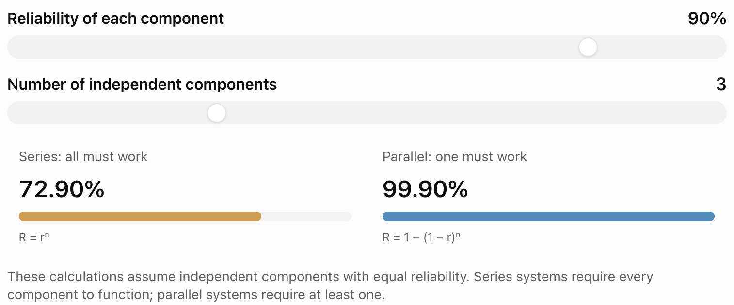
Interactive Reliability Comparison

Explore how component reliability and the number of components affect series and parallel systems.

Exponential Reliability Models

Some engineering components are modelled using an exponential distribution for time until failure.

This model assumes a constant failure rate.

The reliability function is:

R(t) = e^(−λt)

where:

• R(t) is the probability of surviving beyond time t.

• λ is the constant failure rate.

• t is elapsed time.

Worked Example

A component has a constant failure rate of:

λ = 0.002 failures per hour

Find the probability that it operates for at least 100 hours.

R(100) = e^(−0.002 × 100)

= e^(−0.2)

R(100) ≈ 0.8187

There is approximately an 81.87% probability that the component survives beyond 100 hours.

Mean Time to Failure

For an exponential model:

MTTF = 1/λ

For this component:

MTTF = 1/0.002

MTTF = 500 hours

This is the expected time to failure under the model.

Limitations

A constant failure rate may not be realistic for components that wear out with age.

Other models, such as the Weibull distribution, may be more appropriate for systems with changing failure rates.

Probability in Structural Engineering

Structural engineers must consider uncertain loads and material properties.

Examples include:

• Wind forces.

• Vehicle loads.

• Earthquake forces.

• Material strength.

• Construction variations.

A structure is at risk when the applied load exceeds its resistance.

Let:

L = applied load

S = structural strength

Failure occurs when:

L > S

Therefore:

P(failure) = P(L > S)

Simplified Example

Suppose a component can withstand a maximum load of 500 N.

The applied load is normally distributed with:

μ = 400 N

σ = 50 N

Find the probability that the load exceeds 500 N.

Calculate the z-score:

z = (500 − 400)/50

z = 2

From the standard normal distribution:

P(Z > 2) ≈ 0.0228

P(failure) ≈ 2.28%

Interpretation

Under this simplified model, approximately 2.28% of loading events exceed the threshold.

Real structural reliability analysis is more complicated because both load and resistance may vary, and loads may be correlated or change over time.

Probability in Experimental Science

Scientific measurements contain uncertainty.

Repeated measurements of the same quantity may produce slightly different results because of:

• Instrument resolution.

• Environmental variation.

• Random noise.

• Observer differences.

• Experimental conditions.

Probability distributions help describe this variation.

Example: Repeated Measurements

A student measures the length of an object five times.

The results are:

12.1 cm, 12.3 cm, 12.2 cm, 12.0 cm, 12.4 cm

Mean:

x̄ = (12.1 + 12.3 + 12.2 + 12.0 + 12.4)/5

x̄ = 12.2 cm

The measurements vary around the mean.

A standard deviation can be calculated to describe the spread.

Important Distinction

Random measurement variation can often be reduced by taking repeated measurements and averaging.

Systematic errors, such as an incorrectly calibrated instrument, are not necessarily reduced by repetition.

Confidence Intervals in Engineering

A confidence interval estimates an unknown population parameter using sample data.

For a population mean with known population standard deviation σ, a 95% confidence interval is:

x̄ ± 1.96 × σ/√n

where:

• x̄ is the sample mean.

• σ is the population standard deviation.

• n is the sample size.

Worked Example

A factory measures the diameter of 100 components.

The sample mean is:

x̄ = 20.1 mm

The known population standard deviation is:

σ = 0.5 mm

Calculate the standard error:

SE = 0.5/√100

= 0.05 mm

Margin of error:

1.96 × 0.05 = 0.098 mm

Confidence interval:

20.1 ± 0.098

20.002 mm to 20.198 mm

Interpretation

Using this method, approximately 95% of confidence intervals constructed from repeated samples would contain the true population mean, assuming the method's conditions are satisfied.

The interval estimates the mean diameter, not the range containing 95% of individual component diameters.

Monte Carlo Simulation in Engineering

Monte Carlo simulation uses repeated random sampling to investigate uncertain systems.

It is particularly useful when several variables are uncertain.

Example: Manufacturing Dimensions

Suppose the length and width of a manufactured plate vary slightly.

The area is:

A = L × W

If both L and W are uncertain, the area is also uncertain.

A Monte Carlo simulation can:

1. Generate a random length from an appropriate distribution.

2. Generate a random width.

3. Calculate the area.

4. Repeat thousands of times.

5. Analyse the distribution of calculated areas.

The simulation can estimate:

• Mean area.

• Standard deviation of area.

• Probability that area exceeds a limit.

• Probability that area falls within specifications.

Practical Application: Battery Reliability

Suppose a battery-powered system requires two independent batteries connected in parallel.

Each battery has a 95% probability of functioning throughout a mission.

The system works if at least one battery functions.

Probability both batteries fail:

0.05 × 0.05 = 0.0025

System reliability:

R = 1 − 0.0025

R = 0.9975

The system has a 99.75% probability of remaining operational.

Engineering Interpretation

Redundancy improves reliability.

However, if both batteries depend on the same charging system or are exposed to the same extreme temperature, failures may be correlated.

The independence assumption must be evaluated.

Practical Application: Medical Testing

Probability models are important in medical diagnostics.

A test may have:

• Sensitivity: Probability of a positive result when the condition is present.

• Specificity: Probability of a negative result when the condition is absent.

The probability that a person actually has a condition after testing positive also depends on how common the condition is.

Worked Example

Suppose:

• 1% of a population has a particular condition.

• The test has 95% sensitivity.

• The test has 90% specificity.

We want:

P(condition | positive)

Using Bayes' theorem:

P(condition | positive) = P(positive | condition)P(condition) / P(positive)

Calculate:

P(positive) = 0.95 × 0.01 + 0.10 × 0.99

= 0.0095 + 0.099

= 0.1085

Therefore:

P(condition | positive) = 0.0095/0.1085

≈ 0.0876

Approximately 8.76% of positive test results correspond to people who have the condition under these assumptions.

Interpretation

Even a test with relatively high sensitivity can produce many false positives when the condition is uncommon.

This demonstrates why base rates are important in scientific probability.

Practical Application: Environmental Monitoring

Environmental scientists use probability to investigate uncertain natural processes.

Examples include:

• Rainfall.

• Flooding.

• Wind speed.

• Pollution levels.

• Temperature extremes.

• Wildfire occurrence.

Example: Extreme Rainfall

Suppose a simplified model estimates a 5% probability of rainfall exceeding a particular threshold in any given year.

Assume annual exceedance events are independent and the probability remains constant.

The probability of no exceedance over ten years is:

P(no exceedance) = 0.95¹⁰

≈ 0.5987

Therefore:

P(at least one exceedance) = 1 − 0.95¹⁰

≈ 0.4013

There is approximately a 40.13% probability of at least one exceedance during ten years.

Interpretation

A relatively small annual probability can correspond to a much larger probability over a longer period.

This is important when designing infrastructure to withstand rare environmental events.

Interpreting Probabilistic Data

Scientific and engineering results often include probabilities, confidence intervals, and uncertainty estimates.

These values must be interpreted carefully.

Example

An engineer reports:

"The probability of system failure during one year is 0.002."

This means:

P(failure) = 0.002

As a percentage:

0.002 × 100% = 0.2%

The probability of successful operation during the year is:

1 − 0.002 = 0.998

= 99.8%

Important Questions

When interpreting probabilistic data, ask:

• What event is being measured?

• What time period is involved?

• What assumptions were made?

• How were the probabilities estimated?

• Are the events independent?

• Is the sample size sufficient?

• How uncertain are the estimates?

• What are the consequences if the event occurs?

A probability should not be interpreted without its context.

Comparing Engineering Designs

Suppose two engineering designs are available.

Design A

• Cost: $50,000.

• Probability of failure during the first year: 0.04.

• Financial consequence of failure: $100,000.

Expected failure cost:

0.04 × $100,000

= $4,000

Expected total cost:

$50,000 + $4,000

= $54,000

Design B

• Cost: $55,000.

• Probability of failure during the first year: 0.01.

• Financial consequence of failure: $100,000.

Expected failure cost:

0.01 × $100,000

= $1,000

Expected total cost:

$55,000 + $1,000

= $56,000

Comparison

Design A has the lower expected financial cost.

Design B has the lower probability of failure.

Interpretation

If failure could endanger people or cause severe environmental harm, Design B may be preferable despite its higher expected monetary cost.

Engineering decisions must consider safety requirements and consequences, not just expected financial value.

Evaluating Probability Models

Probability models are only useful when their assumptions reasonably represent the system.

Independence

Do component failures occur independently?

Constant Probabilities

Do failure probabilities change with age, temperature, or operating conditions?

Distribution Choice

Does the selected distribution match the observed data?

Sample Quality

Are the observations representative?

Rare Events

Does the model account for uncommon but severe outcomes?

Model Validation

Do predictions agree with real observations?

Sensitivity Analysis

How do results change when uncertain parameters are adjusted?

These questions help determine whether a model is suitable for a scientific or engineering application.

Common Mistakes

Assuming all events are independent

Many engineering failures share common causes.

Using the wrong probability distribution

Counts, measurements, and waiting times may require different models.

Confusing reliability with failure probability

Reliability is the probability of successful operation, while failure probability is its complement over the same period.

Using series reliability formulas for parallel systems

The system structure determines the correct calculation.

Assuming a constant failure rate applies to every component

Some components become more likely to fail as they age.

Confusing expected value with a guaranteed outcome

Expected values describe averages, not certain results.

Misinterpreting confidence intervals

Confidence intervals estimate parameters and must be interpreted according to their construction.

Ignoring systematic measurement errors

Repeated measurements do not automatically remove calibration errors.

Assuming a low annual risk means a low long-term risk

Risk can accumulate over multiple years.

Ignoring the consequences of rare failures

Low-probability events may still be important when their consequences are severe.

Using precise calculations with unrealistic assumptions

Mathematical precision does not guarantee practical accuracy.

Key Terms

• Probability Model: A mathematical representation of uncertain outcomes and their probabilities.

• Random Variable: A numerical variable determined by the outcome of a random process.

• Discrete Random Variable: A random variable with a finite or countably infinite set of values.

• Continuous Random Variable: A random variable that can take any real value within an interval or collection of intervals.

• Deterministic Model: A model producing a fixed result from specified inputs.

• Probabilistic Model: A model incorporating uncertain inputs or outcomes.

• Bernoulli Distribution: A probability model for one success-or-failure trial.

• Binomial Distribution: A model for the number of successes in a fixed number of independent trials.

• Poisson Distribution: A model for the number of events in an interval under appropriate constant-rate assumptions.

• Normal Distribution: A symmetrical, bell-shaped continuous probability distribution.

• Exponential Distribution: A continuous distribution often used for waiting times under a constant event rate.

• Expected Value: The probability-weighted average of possible outcomes.

• Variance: A measure of how widely outcomes are spread around the mean.

• Standard Deviation: The square root of variance, measuring variability in the original units.

• z-Score: The number of standard deviations a value lies above or below the mean.

• Engineering Tolerance: The permitted variation in a manufactured measurement.

• Quality Control: Processes used to assess whether products meet specified standards.

• Defect Probability: The probability that a component fails to meet a required standard.

• Reliability: The probability that a system performs its required function under specified conditions.

• Failure Probability: The probability that a component or system fails during a specified period.

• Series System: A system that requires all components to function.

• Parallel System: A system that functions if at least one alternative component works.

• Redundancy: Additional components or pathways included to improve reliability.

• Failure Rate: A measure describing the frequency or instantaneous tendency of failures.

• Mean Time to Failure (MTTF): The expected operating time before failure.

• Measurement Uncertainty: Uncertainty associated with a measured quantity.

• Sampling Error: Variation caused by estimating a population quantity using a sample.

• Systematic Error: A consistent measurement error caused by bias or calibration problems.

• Confidence Interval: A range calculated using a method designed to contain an unknown parameter at a specified long-run rate.

• Monte Carlo Simulation: A method using repeated random sampling to estimate probabilities or numerical quantities.

• Sensitivity Analysis: An investigation of how model results change when assumptions or parameters change.

• Risk Assessment: The process of evaluating the probability and consequences of uncertain events.

• Model Validation: Comparing model predictions with observations to assess suitability.

Key Takeaways

• Probability models help scientists and engineers analyse uncertain processes and systems.

• Scientific uncertainty may arise from natural randomness, measurement variation, or incomplete information.

• Discrete models are useful for counts, while continuous models are useful for measurements and waiting times.

• Binomial distributions can model the number of defective components under suitable assumptions.

• Poisson distributions can model event counts in fixed intervals.

• Normal distributions are useful for approximately symmetrical measurement variation.

• Expected value describes the average outcome of a random variable.

• Variance and standard deviation measure the spread of possible outcomes.

• Reliability is the probability that a component or system performs successfully for a specified period.

• Series systems require every component to work.

• Parallel systems can continue operating when at least one alternative component works.

• Redundancy can improve reliability when component failures are sufficiently independent.

• Exponential reliability models assume a constant failure rate.

• Manufacturing tolerances can be evaluated using probability distributions.

• Confidence intervals provide estimates of unknown population parameters.

• Monte Carlo simulations can investigate systems with several uncertain variables.

• Bayes' theorem is useful for interpreting diagnostic tests and conditional probabilities.

• Environmental risks may accumulate over time.

• Engineering decisions must consider both the probability and consequences of failure.

• Model assumptions should always be evaluated before interpreting results.

Check Your Understanding

Recall and Understanding

1. Explain why probability is important in science and engineering.

2. Distinguish between deterministic and probabilistic models.

3. Identify three probability distributions commonly used in STEM applications and give an example of each.

4. Define reliability and explain how it differs from failure probability.

5. Explain the difference between series and parallel engineering systems.

Application

6. A factory produces components with a 3% probability of being defective. Assuming independence, calculate the probability that exactly two of 15 components are defective.

7. A radiation detector records an average of four events per minute. Assuming a Poisson model, calculate the probability of recording exactly six events in one minute.

8. A machine component has a constant failure rate of 0.001 per hour. Calculate its reliability after 500 hours.

9. Three independent components in a series system have reliabilities of 0.95, 0.98, and 0.97. Calculate the system reliability.

10. Two independent backup systems each have reliability 0.92. Calculate the reliability of the parallel system.

Analysis and Challenge

11. A manufacturing process produces component lengths that are normally distributed with a mean of 50 mm and a standard deviation of 0.5 mm. Calculate the probability that a component is longer than 51 mm.

12. A structural component can withstand a maximum load of 800 N. Applied loads are normally distributed with a mean of 650 N and a standard deviation of 75 N. Estimate the probability that the load exceeds the component's capacity.

13. A factory is comparing two engineering designs. Design A costs $40,000 with a 5% probability of a $100,000 failure. Design B costs $45,000 with a 1% probability of the same failure. Calculate the expected total cost of each design and justify which may be preferable.

14. A flood has a 2% probability of exceeding a specified level in any given year. Assuming independence, calculate the probability of at least one exceedance during the next 25 years. Explain why this matters for infrastructure planning.

15. Design a probability model for a real-world STEM application. Identify the random variable, select an appropriate distribution, state the assumptions, perform a probability calculation, and explain how the results could inform a scientific or engineering decision.

Final Summary

Probability is an essential mathematical tool in science and engineering because real systems involve uncertainty.

Probability distributions help model random events, measurement variation, manufacturing defects, equipment failures, and environmental processes.

Reliability engineering uses probability to estimate whether components and systems will operate successfully under specified conditions.

Series and parallel reliability models demonstrate how system structure affects overall performance.

Statistical methods, including confidence intervals and Monte Carlo simulation, allow scientists and engineers to interpret uncertain data and investigate complex systems.

Probability also supports practical decisions involving quality control, safety, infrastructure, medical testing, and environmental risk.

The central principle is that probability does not eliminate uncertainty. Instead, it provides a mathematical framework for understanding uncertainty, estimating risk, and making better-informed scientific and engineering decisions.