Applications of Probability and Combinatoric
1. Decision Making Under Uncertainty
Learning outcomes
- I can apply expected value to decision making.
- I can compare risks and rewards.
- I can analyse uncertain outcomes.
- I can evaluate alternative strategies.
- I can justify decisions mathematically.
Decision Making Under Uncertainty
Introduction to Decision Making Under Uncertainty
Every day, individuals, businesses, scientists, and governments make decisions without knowing exactly what will happen.
For example:
-
Should a company invest in a new product?
-
Is it better to repair an old machine or purchase a new one?
-
How much stock should a shop order when customer demand is uncertain?
-
Should a farmer plant a crop that produces higher profits but is more vulnerable to drought?
-
Which transportation option offers the best balance between cost, reliability, and travel time?
These decisions involve uncertainty, because several outcomes are possible and the final result cannot be predicted with certainty.
Mathematics provides methods for comparing these alternatives.
One of the most important tools is expected value, which combines possible outcomes with their probabilities to calculate a probability-weighted average.
However, a good decision may also depend on risk, the severity of possible losses, available resources, and the consequences of different outcomes.
Decision making under uncertainty involves using probability, expected value, and mathematical reasoning to compare alternatives and select an appropriate course of action.


Understanding Uncertainty and Risk
Although the words risk and uncertainty are often used together, they have slightly different meanings in decision analysis.
Risk describes situations where different outcomes are possible and their probabilities can be estimated.
Uncertainty is a broader term describing situations where the future is unknown. In some cases, even the probabilities of different outcomes may be difficult to estimate.
Examples
|
Situation |
Possible outcomes |
Source of uncertainty |
|---|---|---|
|
Launching a product |
High, moderate, or low sales |
Customer demand |
|
Planting crops |
High or low harvest |
Weather and growing conditions |
|
Purchasing equipment |
Reliable operation or breakdown |
Equipment performance |
|
Planning an event |
High or low attendance |
Customer participation |
|
Choosing transportation |
Early, on-time, or late arrival |
Traffic and service delays |
In many mathematical problems, probabilities are provided or can be estimated from data.
These probabilities allow us to calculate expected outcomes.
Expected Value
The expected value of a random variable is the probability-weighted average of its possible outcomes.
For a discrete random variable X:
E(X) = Σ[x × P(X = x)]
where:
-
E(X) is the expected value.
-
x is a possible numerical outcome.
-
P(X = x) is the probability of that outcome.
-
Σ means to add the products for all possible outcomes.
Interpretation
Expected value represents the long-run average outcome if the same decision or random experiment were repeated many times under the same conditions.
It does not necessarily represent an outcome that will actually occur.
For example, the expected number of heads in three fair coin tosses is 1.5.
However, obtaining exactly 1.5 heads is impossible.
Expected value is an average, not a guaranteed result.
Worked Example: Expected Profit
Suppose a company is considering launching a small product.
The possible profits are:
|
Outcome |
Probability |
Profit |
|---|---|---|
|
High sales |
0.30 |
$20,000 |
|
Moderate sales |
0.50 |
$8,000 |
|
Low sales |
0.20 |
−$5,000 |
A negative profit represents a loss.
Step 1: Multiply Each Outcome by Its Probability
High sales:
0.30 × $20,000 = $6,000
Moderate sales:
0.50 × $8,000 = $4,000
Low sales:
0.20 × (−$5,000) = −$1,000
Step 2: Add the Results
E(X) = $6,000 + $4,000 − $1,000
E(X) = $9,000
Interpretation
The expected profit is $9,000.
This does not mean the company will earn exactly $9,000.
The actual outcome could be a $20,000 profit, an $8,000 profit, or a $5,000 loss.
The expected value provides a mathematical summary of the possible outcomes and their probabilities.
Expected Monetary Value
When outcomes are measured in money, expected value is often called expected monetary value (EMV).
EMV = Σ[Probability × Monetary outcome]
EMV can be used to compare:
-
Investment opportunities.
-
Business strategies.
-
Equipment purchases.
-
Insurance decisions.
-
Product launches.
-
Project alternatives.
If the objective is to maximize expected monetary gain, the strategy with the highest EMV is preferred.
However, maximizing EMV does not always produce the most suitable decision when financial losses or other consequences are significant.
Comparing Alternative Strategies
Suppose a company is choosing between two business strategies.
Strategy A: Conservative Expansion
|
Outcome |
Probability |
Profit |
|---|---|---|
|
Successful expansion |
0.80 |
$12,000 |
|
Unsuccessful expansion |
0.20 |
−$2,000 |
Expected value:
EMV(A) = 0.80 × $12,000 + 0.20 × (−$2,000)
= $9,600 − $400
EMV(A) = $9,200
Strategy B: Aggressive Expansion
|
Outcome |
Probability |
Profit |
|---|---|---|
|
Successful expansion |
0.40 |
$30,000 |
|
Unsuccessful expansion |
0.60 |
−$4,000 |
Expected value:
EMV(B) = 0.40 × $30,000 + 0.60 × (−$4,000)
= $12,000 − $2,400
EMV(B) = $9,600
Comparing the Results
|
Measure |
Strategy A |
Strategy B |
|---|---|---|
|
Expected profit |
$9,200 |
$9,600 |
|
Maximum profit |
$12,000 |
$30,000 |
|
Maximum loss |
$2,000 |
$4,000 |
|
Probability of loss |
20% |
60% |
Strategy B has the higher expected profit.
However, it also has a higher probability of loss and a larger potential loss.
A company focused on maximizing expected profit may prefer Strategy B.
A company concerned about financial stability may prefer Strategy A.
The mathematically preferred decision depends on the objective and the constraints of the decision-maker.
Comparing Risks and Rewards
Expected value is important, but it does not fully describe risk.
Two strategies may have the same expected value while producing very different outcomes.
Example
Consider two options.
Option A
Receive $500 with certainty.
Expected value:
E(A) = $500
Option B
-
50% probability of receiving $1,200.
-
50% probability of losing $200.
Expected value:
E(B) = 0.50 × $1,200 + 0.50 × (−$200)
= $600 − $100
E(B) = $500
Both options have the same expected value.
However, Option A guarantees $500, while Option B involves substantial uncertainty.
Interpretation
A risk-averse person may prefer Option A.
A person willing to accept uncertainty for the possibility of a larger reward may prefer Option B.
Neither preference is automatically mathematically incorrect.
Expected value is only one part of the decision.
Variance and Standard Deviation in Decision Making
The variance of a random variable measures how widely possible outcomes are spread around the expected value.
For a discrete random variable:
Var(X) = Σ[(x − μ)² × P(X = x)]
where:
μ = E(X)
The standard deviation is:
σ = √Var(X)
A larger standard deviation indicates greater variability in possible outcomes.
Worked Example: Comparing Two Options
Consider the previous options.
Option A guarantees $500.
Therefore:
E(A) = $500
Var(A) = 0
σ(A) = 0
Option B offers:
-
$1,200 with probability 0.5.
-
−$200 with probability 0.5.
Its expected value is $500.
Calculate the variance:
Var(B) = 0.5 × (1200 − 500)² + 0.5 × (−200 − 500)²
= 0.5 × 700² + 0.5 × (−700)²
= 245,000 + 245,000
Var(B) = 490,000
Standard deviation:
σ(B) = √490000
σ(B) = $700
Interpretation
Both options have the same expected value, but Option B has a much larger standard deviation.
This means its possible outcomes vary more widely around the expected value.
Standard deviation provides a useful measure of risk when comparing outcomes on the same scale.
Decision Tables
A decision table, also called a payoff table, organizes possible decisions and their outcomes under different conditions.
Suppose a shop must decide how much stock to order.
The shop has two options:
-
Order 100 units.
-
Order 200 units.
Customer demand may be:
-
Low
-
High
The profits are:
|
Decision |
Low demand |
High demand |
|---|---|---|
|
Order 100 units |
$1,000 |
$1,000 |
|
Order 200 units |
−$500 |
$2,500 |
Suppose:
P(low demand) = 0.40
P(high demand) = 0.60
Expected Value of Ordering 100 Units
EMV(100) = 0.40 × $1,000 + 0.60 × $1,000
EMV(100) = $1,000
Expected Value of Ordering 200 Units
EMV(200) = 0.40 × (−$500) + 0.60 × $2,500
= −$200 + $1,500
EMV(200) = $1,300
Decision
Ordering 200 units has the higher expected profit.
However, ordering 100 units avoids the possibility of a loss under the two scenarios.
The appropriate decision depends on whether maximizing expected profit or limiting financial risk is more important.

Decision Trees
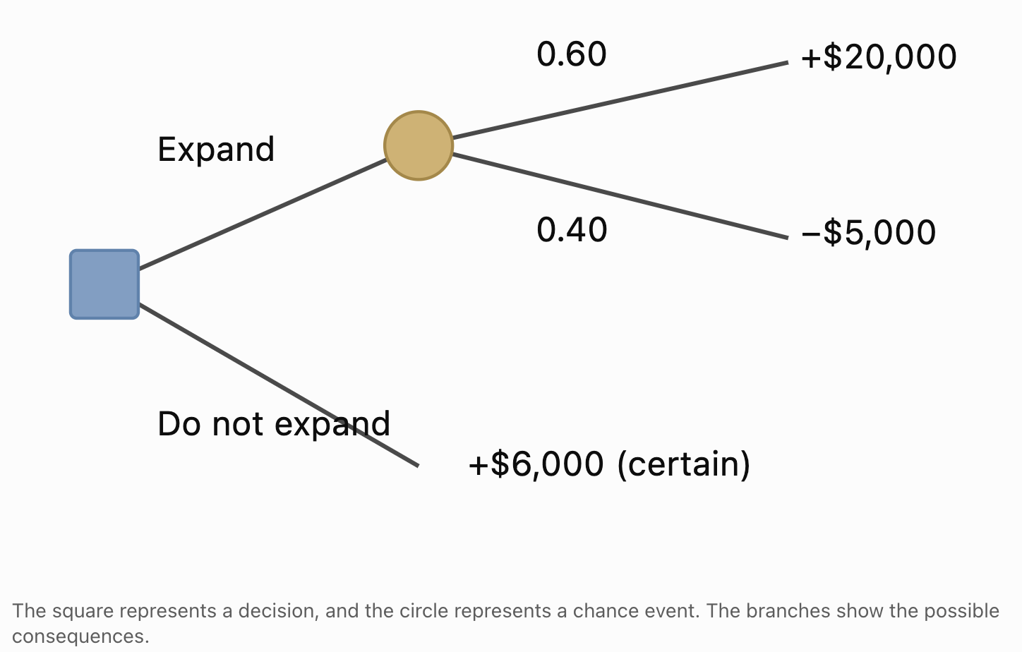
A decision tree is a diagram showing possible decisions, uncertain events, and their consequences.
Decision trees are useful when a problem involves several stages.
Two common types of nodes are:
-
Decision nodes: Points where a choice is made, often represented by squares.
-
Chance nodes: Points where an uncertain outcome occurs, often represented by circles.
Example: Business Expansion
A company must decide whether to expand.
If it expands:
-
There is a 60% probability of earning $20,000.
-
There is a 40% probability of losing $5,000.
If it does not expand:
- The profit is $6,000.
Step 1: Calculate the Expected Value of Expanding
EMV(expand) = 0.60 × $20,000 + 0.40 × (−$5,000)
= $12,000 − $2,000
EMV(expand) = $10,000
Step 2: Calculate the Value of Not Expanding
EMV(do not expand) = $6,000
Step 3: Compare
|
Decision |
Expected profit |
|---|---|
|
Expand |
$10,000 |
|
Do not expand |
$6,000 |
Expanding has the higher expected monetary value.
Decision
If the company wants to maximize expected profit and can tolerate the possible loss, expanding is the preferred strategy.
If avoiding losses is essential, not expanding may be more appropriate.
Analysing Decisions with Several Stages
Some decisions involve a sequence of uncertain events.
For example, a company might:
-
Invest in product development.
-
Conduct a market test.
-
Decide whether to launch the product.
-
Experience high or low customer demand.
Decision trees can represent these stages.
Solving Multi-Stage Decision Trees
A common method is rollback analysis.
Start at the final outcomes and work backward.
At each chance node:
Calculate the probability-weighted expected value.
At each decision node:
Choose the alternative with the preferred value according to the decision criterion.
Continue backward until reaching the initial decision.
This allows complex decisions to be evaluated systematically.
Risk Attitudes
People and organizations differ in how they respond to uncertain outcomes.
Three common attitudes toward risk are:
Risk-Averse
A risk-averse decision-maker prefers greater certainty when alternatives have the same expected value.
For example, they may prefer a guaranteed $500 over a risky option with an expected value of $500.
Risk-Neutral
A risk-neutral decision-maker evaluates alternatives primarily according to expected monetary value.
If two options have the same expected value, they are equally attractive under this criterion.
Risk-Seeking
A risk-seeking decision-maker may prefer an uncertain option over a guaranteed option with the same expected value.
The possibility of a large reward may be especially attractive.
Important Principle
Risk attitudes influence decisions, but they do not change the mathematical expected values of the alternatives.
Expected Utility
Expected monetary value is not always enough to describe preferences.
For example, losing $10,000 may have a very different impact on a small business than on a large corporation.
Utility is a mathematical representation of how desirable an outcome is to a decision-maker.
Expected utility is calculated using:
E[U(X)] = Σ[P(X = x) × U(x)]
where:
U(x) represents the utility of outcome x.
A decision-maker can compare alternatives using expected utility rather than expected money alone.
Example
A person may value financial security more highly than the possibility of earning a much larger amount.
A utility function can represent that preference.
Expected utility provides a more flexible framework for decision-making when risk attitudes matter.
The Value of Information
Sometimes a decision-maker can obtain additional information before making a decision.
For example:
-
A company might conduct market research.
-
A farmer might purchase a detailed weather forecast.
-
A manufacturer might inspect equipment.
-
A doctor might request an additional diagnostic test.
Information can improve decisions by reducing uncertainty.
Expected Value of Perfect Information
The expected value of perfect information (EVPI) measures how much better the expected outcome could be if the decision-maker knew the future state before choosing.
EVPI = Expected value with perfect information − Best expected value without perfect information
EVPI represents the maximum amount a risk-neutral decision-maker should be willing to pay for perfect information under the model.
Worked Example: Value of Market Research
Consider the earlier stock-ordering problem.
|
Decision |
Low demand |
High demand |
|---|---|---|
|
Order 100 units |
$1,000 |
$1,000 |
|
Order 200 units |
−$500 |
$2,500 |
Probabilities:
P(low demand) = 0.40
P(high demand) = 0.60
The best expected value without additional information is:
$1,300
With Perfect Information
If the shop knew demand would be low, it would order 100 units and earn $1,000.
If it knew demand would be high, it would order 200 units and earn $2,500.
Expected value with perfect information:
EV(with perfect information) = 0.40 × $1,000 + 0.60 × $2,500
= $400 + $1,500
= $1,900
Calculate EVPI
EVPI = $1,900 − $1,300
EVPI = $600
Interpretation
Perfect information would increase expected profit by $600.
Therefore, under this model, a risk-neutral shop owner should not pay more than $600 for perfect information.
Real market research is imperfect, so its expected value would generally be lower.
Decisions When Probabilities Are Unknown
Sometimes probabilities cannot be estimated reliably.
In these situations, expected value may not be appropriate.
Alternative decision criteria can be used.
Maximax Criterion
Choose the strategy with the highest possible payoff.
This is an optimistic approach.
Maximin Criterion
Choose the strategy with the highest worst-case payoff.
This is a conservative approach.
Minimax Regret Criterion
Choose the strategy that minimizes the largest possible regret.
Regret is the difference between the best payoff that could have been obtained in a particular state and the payoff from the chosen strategy.
Example
|
Strategy |
Low demand |
High demand |
|---|---|---|
|
A |
$5,000 |
$10,000 |
|
B |
−$2,000 |
$20,000 |
|
C |
$3,000 |
$14,000 |
Maximax: Strategy B, because its maximum payoff is $20,000.
Maximin: Strategy A, because its minimum payoff is $5,000, higher than the minimum payoffs of the other strategies.
For minimax regret:
-
Under low demand, the best payoff is $5,000.
-
Under high demand, the best payoff is $20,000.
|
Strategy |
Regret under low demand |
Regret under high demand |
Maximum regret |
|---|---|---|---|
|
A |
$0 |
$10,000 |
$10,000 |
|
B |
$7,000 |
$0 |
$7,000 |
|
C |
$2,000 |
$6,000 |
$6,000 |
Minimax regret: Strategy C, because its maximum regret is the smallest.
Different decision criteria can produce different choices.
Sensitivity Analysis in Decision Making
Decision models depend on estimated probabilities.
If these probabilities change, the preferred strategy may also change.
Sensitivity analysis examines how changes in assumptions affect the decision.
Worked Example
Suppose a company is considering a project.
If successful, the project earns $15,000.
If unsuccessful, it loses $5,000.
Let p be the probability of success.
Expected value:
EMV = 15000p − 5000(1 − p)
Expand:
EMV = 15000p − 5000 + 5000p
EMV = 20000p − 5000
Find the Break-Even Probability
Set expected value equal to zero:
20000p − 5000 = 0
20000p = 5000
p = 0.25
Interpretation
-
If p > 0.25, the expected profit is positive.
-
If p = 0.25, the expected profit is zero.
-
If p < 0.25, the expected profit is negative.
The break-even success probability is 25%.
This result helps the company evaluate whether its estimate of the probability of success is sufficiently high.
Comparing Strategies Across Different Probabilities
Using the previous example:
EMV = 20000p − 5000
|
Probability of success |
Expected profit |
|---|---|
|
10% |
−$3,000 |
|
20% |
−$1,000 |
|
25% |
$0 |
|
40% |
$3,000 |
|
60% |
$7,000 |
|
80% |
$11,000 |
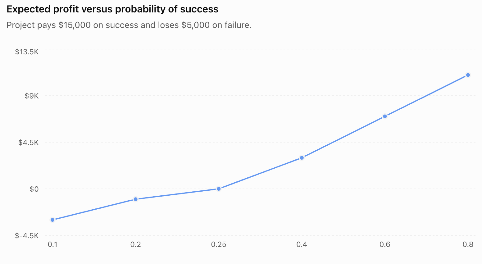
The graph illustrates how the expected profit increases as the probability of success increases.
Sensitivity analysis is especially useful when probabilities are uncertain or based on limited data.
Practical Application: Equipment Replacement
A factory must decide whether to continue using an older machine or purchase a replacement.
Keep the Old Machine
-
70% probability of no major breakdown, costing $2,000 in maintenance.
-
30% probability of a breakdown, costing $18,000 in total.
Expected cost:
E(C_old) = 0.70 × $2,000 + 0.30 × $18,000
= $1,400 + $5,400
E(C_old) = $6,800
Purchase a New Machine
Suppose the new machine has a total annualized cost of $6,000, including purchase-related costs and expected maintenance.
Expected cost:
E(C_new) = $6,000
Decision
|
Option |
Expected cost |
|---|---|
|
Keep old machine |
$6,800 |
|
Purchase new machine |
$6,000 |
Purchasing the new machine has the lower expected cost by $800.
However, the company should also consider equipment lifespan, downtime, productivity, and the accuracy of the cost estimates.

Practical Application: Agricultural Decisions
A farmer must choose between two crops.
Crop A produces relatively stable profits.
Crop B can produce much higher profits in favourable weather but performs poorly during drought.
Suppose:
|
Weather |
Probability |
Crop A profit |
Crop B profit |
|---|---|---|---|
|
Good rainfall |
0.60 |
$12,000 |
$20,000 |
|
Drought |
0.40 |
$6,000 |
−$4,000 |
Expected Profit for Crop A
EMV(A) = 0.60 × $12,000 + 0.40 × $6,000
= $7,200 + $2,400
EMV(A) = $9,600
Expected Profit for Crop B
EMV(B) = 0.60 × $20,000 + 0.40 × (−$4,000)
= $12,000 − $1,600
EMV(B) = $10,400
Crop B has the higher expected profit.
However, Crop A provides a positive profit under both weather conditions.
A farmer with limited financial reserves may reasonably prefer Crop A.

Practical Application: Transportation Choices
Suppose a student can travel to school using either a bus or a train.
Bus
-
70% probability of arriving in 25 minutes.
-
30% probability of arriving in 45 minutes.
Expected travel time:
E(T_bus) = 0.70 × 25 + 0.30 × 45
= 17.5 + 13.5
E(T_bus) = 31 minutes
Train
-
90% probability of arriving in 30 minutes.
-
10% probability of arriving in 40 minutes.
Expected travel time:
E(T_train) = 0.90 × 30 + 0.10 × 40
= 27 + 4
E(T_train) = 31 minutes
Both options have the same expected travel time.
However, the train has less variation in travel time.
A student who must arrive before a strict deadline may prefer the train.
This example demonstrates why expected value alone may not determine the best choice.
Communicating Mathematical Decisions
A well-justified decision should explain both the calculations and the reasoning behind the recommendation.
A Strong Mathematical Justification Includes
-
A clear statement of the decision.
-
The available alternatives.
-
Possible outcomes and their probabilities.
-
Expected value calculations.
-
Relevant measures of risk.
-
Assumptions and limitations.
-
A conclusion that matches the decision objective.
Example
"Strategy B has an expected profit of $9,600, compared with $9,200 for Strategy A. Therefore, Strategy B is preferable if the objective is to maximize expected profit. However, Strategy B also has a 60% probability of loss, compared with 20% for Strategy A. A company prioritizing financial stability may therefore prefer Strategy A despite its slightly lower expected value."
This explanation is stronger than simply stating that Strategy B is better.
It recognises both expected reward and risk.
Limitations of Mathematical Decision Models
Mathematical models help organize uncertain decisions, but they have limitations.
Estimated Probabilities May Be Incorrect
Probabilities are often based on historical data or assumptions.
Future conditions may differ from the past.
Outcomes May Be Incomplete
Some important consequences may be difficult to measure financially.
For example:
-
Environmental damage.
-
Safety risks.
-
Reputation.
-
Customer satisfaction.
-
Social consequences.
Decision-Makers Have Different Objectives
One person may prioritize maximum expected profit.
Another may prioritize avoiding severe losses.
Rare Events Can Have Major Consequences
An event with a small probability may still require serious attention if its consequences are extremely harmful.
Conditions May Change
Market demand, weather, technology, and other factors can change over time.
Decision models should be reviewed when new information becomes available.
Common Mistakes
Assuming the highest expected value is always the best decision
Expected value does not fully describe risk, financial constraints, or personal preferences.
Ignoring negative outcomes
Losses must be included using negative values when calculating expected profit.
Forgetting to multiply outcomes by probabilities
Expected value is a weighted average, not a simple average unless outcomes are equally likely.
Using probabilities that do not add to 1
A complete probability distribution must have total probability equal to 1.
Confusing expected value with a guaranteed outcome
The expected value may never occur in a single trial.
Ignoring the probability of severe losses
A strategy may have a high expected value while exposing the decision-maker to unacceptable risks.
Confusing variance and standard deviation
Variance is measured in squared units, while standard deviation uses the original units.
Comparing costs and profits incorrectly
When evaluating profits, larger expected values are generally preferred. When evaluating costs, smaller expected values are generally preferred.
Assuming perfect information is free
Obtaining information may involve financial costs and delays.
Failing to consider uncertain probabilities
Sensitivity analysis is important when probability estimates may be inaccurate.
Providing a decision without mathematical justification
A strong conclusion should include calculations, assumptions, and interpretation.
Key Terms
-
Decision Making Under Uncertainty: Choosing between alternatives when future outcomes are not known with certainty.
-
Risk: Exposure to uncertain outcomes whose probabilities can be estimated.
-
Uncertainty: Lack of certainty about future events or outcomes.
-
Expected Value: The probability-weighted average of possible numerical outcomes.
-
Expected Monetary Value (EMV): Expected value when outcomes are expressed in money.
-
Payoff: The result or reward associated with a decision and a particular outcome.
-
Payoff Table: A table organizing possible decisions and their outcomes.
-
Decision Tree: A diagram representing decisions, uncertain events, and possible consequences.
-
Decision Node: A point in a decision tree where a choice must be made.
-
Chance Node: A point in a decision tree where an uncertain event occurs.
-
Rollback Analysis: A method of solving decision trees by working backward from final outcomes.
-
Variance: A measure of how widely possible outcomes are spread around their expected value.
-
Standard Deviation: The square root of variance, measuring variability in the original units.
-
Risk-Averse: Preferring greater certainty when alternatives have the same expected value.
-
Risk-Neutral: Evaluating alternatives primarily according to expected monetary value.
-
Risk-Seeking: Preferring greater uncertainty when alternatives have the same expected value.
-
Utility: A numerical representation of how desirable an outcome is to a decision-maker.
-
Expected Utility: The probability-weighted average of the utilities of possible outcomes.
-
Value of Information: The improvement in expected decision outcomes made possible by additional information.
-
Expected Value of Perfect Information (EVPI): The maximum expected improvement achievable by knowing the future state before making a decision.
-
Maximax Criterion: A decision rule that selects the alternative with the highest possible payoff.
-
Maximin Criterion: A decision rule that selects the alternative with the highest worst-case payoff.
-
Minimax Regret: A decision rule that minimizes the largest possible regret.
-
Regret: The difference between the best available payoff in a particular state and the payoff from the selected strategy.
-
Sensitivity Analysis: An investigation of how changes in assumptions affect decision outcomes.
-
Break-Even Probability: The probability at which an expected payoff or the difference between strategies reaches zero.
-
Opportunity Cost: The value of the best alternative forgone when a decision is made.
-
Mathematical Justification: An explanation supporting a decision using calculations, assumptions, and logical reasoning.
Key Takeaways
-
Expected value is a powerful tool for comparing decisions involving uncertain outcomes.
-
Expected value is calculated by multiplying each possible outcome by its probability and adding the results.
-
Expected monetary value applies expected value to financial decisions.
-
A higher expected value does not guarantee a better outcome in any single situation.
-
Expected value represents a long-run average under the assumptions of the model.
-
Risk and reward should be considered together.
-
Variance and standard deviation measure the variability of possible outcomes.
-
Two alternatives can have the same expected value but different levels of risk.
-
Decision tables organize alternative strategies and possible outcomes.
-
Decision trees represent sequences of decisions and uncertain events.
-
Rollback analysis evaluates multi-stage decisions by working backward.
-
Risk-averse, risk-neutral, and risk-seeking decision-makers may prefer different strategies.
-
Expected utility can represent preferences that expected monetary value alone does not capture.
-
Additional information can improve decisions by reducing uncertainty.
-
EVPI measures the maximum expected benefit of perfect information.
-
When probabilities are unknown, maximax, maximin, and minimax regret provide alternative decision criteria.
-
Sensitivity analysis shows how changes in probabilities affect expected outcomes.
-
Break-even probabilities identify thresholds where a decision becomes financially favourable.
-
Mathematical decisions should consider assumptions, limitations, and possible consequences.
-
A strong mathematical justification explains the calculations and why the recommended strategy fits the decision objective.
Check Your Understanding
Recall and Understanding
-
Define expected value and explain how it is used in decision making.
-
Explain the difference between risk and uncertainty.
-
Describe the purpose of a decision tree.
-
Explain why two strategies with the same expected value may not be equally attractive.
-
Distinguish between risk-averse, risk-neutral, and risk-seeking decision-makers.
Application
-
A project has a 60% probability of earning $10,000 and a 40% probability of losing $3,000. Calculate its expected monetary value.
-
Strategy A guarantees a profit of $4,000. Strategy B offers a 50% probability of earning $10,000 and a 50% probability of losing $1,000. Compare their expected values.
-
A company can purchase a machine with an expected annual operating cost of $5,000 or keep an older machine with a 70% probability of costing $3,000 and a 30% probability of costing $12,000. Determine which option has the lower expected cost.
-
A decision has two outcomes: a $2,000 profit with probability 0.8 and a $3,000 loss with probability 0.2. Calculate the expected value and standard deviation.
-
A project earns $8,000 if successful and loses $2,000 if unsuccessful. Find the minimum probability of success required for a positive expected profit.
Analysis and Challenge
-
A company must choose between two strategies. Strategy A has an expected profit of $15,000 and a standard deviation of $2,000. Strategy B has an expected profit of $18,000 and a standard deviation of $10,000. Explain which strategy may be preferable for different risk attitudes.
-
A shop can order either 50 or 100 products. Construct a payoff table using reasonable assumptions about demand, calculate expected profits, and justify the preferred order quantity.
-
A business can conduct market research before launching a product. Explain how the expected value of perfect information could help determine whether the research is worth purchasing.
-
A project has a 40% probability of earning $20,000 and a 60% probability of losing $5,000. Calculate its expected value. Then explain how the decision might change if the probability of success were uncertain.
-
Design a real-world decision problem involving at least three possible outcomes and two alternative strategies. Construct a payoff table, calculate expected values, compare risks, and justify your recommended decision.
Final Summary
Decision making under uncertainty involves selecting between alternatives when future outcomes cannot be predicted with certainty.
Expected value provides a mathematical method for comparing strategies by combining possible outcomes with their probabilities.
However, expected value alone does not describe the full range of possible consequences.
Measures such as variance and standard deviation help quantify risk, while decision trees, payoff tables, and sensitivity analysis provide additional tools for evaluating alternatives.
Different decision-makers may choose different strategies because they have different objectives, resources, and attitudes toward risk.
The most effective decisions combine mathematical calculations with careful consideration of assumptions, uncertainty, and practical consequences.
A well-justified decision is not simply the one with the highest expected value. It is the decision that best meets the objective while accounting for the risks and limitations of the available information.