Advanced Probability
1. Bayes' Theorem
Learning outcomes
- I can explain Bayes' Theorem.
- I can calculate posterior probabilities.
- I can interpret Bayesian reasoning.
- I can solve diagnostic testing problems.
- I can apply Bayesian thinking to real-world situations.
Bayes' Theorem
Introduction to Bayes' Theorem
In everyday life, we often make decisions using incomplete information. When new evidence becomes available, we may need to reconsider what we previously believed.
For example:
-
A medical test produces a positive result. How likely is it that the patient actually has the condition?
-
A factory inspection identifies a defective product. Which machine most likely produced it?
-
An email is flagged as spam. How likely is it to be unwanted?
-
A weather forecast predicts rain. How should new weather observations change that prediction?
-
A scientific experiment produces unexpected results. How should researchers update their hypotheses?
These situations involve conditional probability and Bayesian reasoning.
Bayes' Theorem is a mathematical rule that allows us to update the probability of an event when new evidence becomes available.
It connects what we believed before observing the evidence with what we should believe after considering it.


Reviewing Conditional Probability
Before studying Bayes' Theorem, it is important to understand conditional probability.
A conditional probability describes the probability of an event occurring when another event is already known to have occurred.
It is written as:
P(A | B)
This is read as:
"The probability of A given B."
For example:
-
A = a student passes an examination.
-
B = the student attended a revision session.
Then:
P(A | B)
represents the probability that a student passes the examination, given that the student attended the revision session.
Conditional Probability Formula
P(A | B) = P(A ∩ B)/P(B)
where:
-
P(A | B) is the probability of A given B.
-
P(A ∩ B) is the probability that both A and B occur.
-
P(B) is the probability of B.
This formula requires P(B) > 0.
Worked Example: Students and Sports
Suppose a school has 100 students.
-
40 students play basketball.
-
30 students play football.
-
15 students play both sports.
Let:
A = student plays basketball
B = student plays football
Find the probability that a student plays basketball, given that the student plays football.
P(A | B) = P(A ∩ B)/P(B)
= (15/100)/(30/100)
= 15/30
P(A | B) = 0.5
There is a 50% probability that a student plays basketball, given that the student plays football.
Why Conditional Probabilities Are Different
One of the most important ideas in Bayesian reasoning is that:
P(A | B) is not generally equal to P(B | A).
For example:
-
P(positive test | disease) describes how often a test correctly identifies people who have a disease.
-
P(disease | positive test) describes how likely a person is to have the disease after receiving a positive result.
These probabilities answer different questions.
A medical test can correctly identify most people with a disease while many positive results still occur among people who do not have the disease.
Understanding this distinction is essential for interpreting diagnostic tests, scientific evidence, and statistical claims.
Understanding Bayes' Theorem
Bayes' Theorem provides a method for reversing conditional probabilities.
The formula is:
P(A | B) = [P(B | A) × P(A)]/P(B)
where:
-
P(A | B) is the probability of A after observing B.
-
P(B | A) is the probability of observing B if A is true.
-
P(A) is the probability of A before observing B.
-
P(B) is the overall probability of observing B.
The formula requires P(B) > 0.
Understanding the Components
Bayes' Theorem can be expressed conceptually as:
Posterior probability = Likelihood × Prior probability / Evidence probability
Each part has a specific meaning.
|
Term |
Meaning |
|---|---|
|
Prior probability |
Initial probability before new evidence |
|
Likelihood |
Probability of observing the evidence if the hypothesis is true |
|
Evidence probability |
Overall probability of observing the evidence |
|
Posterior probability |
Updated probability after considering the evidence |
Bayes' Theorem describes how evidence changes our estimate of a probability.
Prior and Posterior Probabilities
Prior Probability
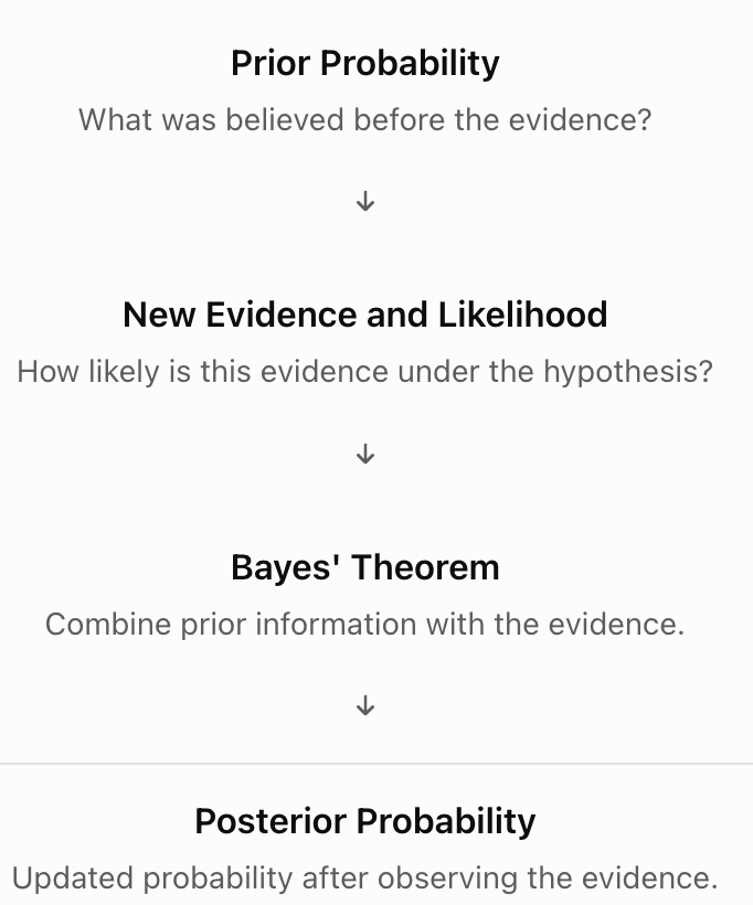
The prior probability is the probability assigned to an event before considering new evidence.
For example, suppose 5% of manufactured products are defective.
Before inspecting a randomly selected product:
P(defective) = 0.05
This is the prior probability.
Posterior Probability
The posterior probability is the updated probability after considering new evidence.
Suppose an inspection system identifies the product as potentially defective.
We can use Bayes' Theorem to determine the probability that the product is actually defective, given the inspection result.
Bayesian Updating
The process can be summarized as:
The Law of Total Probability
Bayes' Theorem often requires calculating the overall probability of the evidence.
Suppose A and not A are the only two possibilities.
Then:
P(B) = P(B | A)P(A) + P(B | not A)P(not A)
This is an application of the Law of Total Probability.
It considers two different ways that event B can occur:
-
B occurs when A is true.
-
B occurs when A is false.
The probabilities of these two mutually exclusive possibilities are added.
Expanded Form of Bayes' Theorem
Substituting the total probability formula gives:
P(A | B) = [P(B | A)P(A)]/[P(B | A)P(A) + P(B | not A)P(not A)]
This form is particularly useful for diagnostic testing problems.
Worked Example: A Simple Bayesian Calculation
Suppose a factory produces electronic components.
-
10% of components are defective.
-
An inspection system flags 90% of defective components.
-
The system also flags 20% of non-defective components.
A component is flagged.
What is the probability that it is actually defective?
Step 1: Define the Events
Let:
D = component is defective
F = component is flagged
We know:
P(D) = 0.10
P(not D) = 0.90
P(F | D) = 0.90
P(F | not D) = 0.20
We want:
P(D | F)
Step 2: Calculate the Overall Probability of Being Flagged
P(F) = P(F | D)P(D) + P(F | not D)P(not D)
= (0.90 × 0.10) + (0.20 × 0.90)
= 0.09 + 0.18
P(F) = 0.27
Step 3: Apply Bayes' Theorem
P(D | F) = [P(F | D)P(D)]/P(F)
= (0.90 × 0.10)/0.27
= 0.09/0.27
P(D | F) ≈ 0.3333
Interpretation
There is approximately a 33.33% probability that a flagged component is actually defective.
Although the inspection system detects 90% of defective components, many flagged components are not defective because non-defective components are much more common.
This demonstrates why the prior probability matters.
Understanding Bayesian Reasoning with Frequency Tables
Bayesian calculations can become easier to understand when probabilities are converted into expected frequencies.
Using the previous example, suppose the factory produces 1,000 components.
Step 1: Determine the Number of Defective Components
10% are defective.
1,000 × 0.10 = 100
Therefore:
-
100 components are defective.
-
900 components are non-defective.
Step 2: Apply the Inspection Results
Of the 100 defective components:
90% are flagged.
100 × 0.90 = 90
Of the 900 non-defective components:
20% are flagged.
900 × 0.20 = 180
Step 3: Construct a Table
|
Actual condition |
Flagged |
Not flagged |
Total |
|---|---|---|---|
|
Defective |
90 |
10 |
100 |
|
Non-defective |
180 |
720 |
900 |
|
Total |
270 |
730 |
1,000 |
Step 4: Calculate the Posterior Probability
Of the 270 flagged components, 90 are actually defective.
P(defective | flagged) = 90/270
P(defective | flagged) = 1/3 ≈ 33.33%
The frequency-table method produces the same result as Bayes' Theorem.

Bayes' Theorem and Diagnostic Testing
One of the most important applications of Bayes' Theorem is interpreting diagnostic tests.
A diagnostic test may be used to identify a medical condition.
However, test results are not always correct.
Two important measures describe test performance.
Sensitivity
Sensitivity is the probability that a test gives a positive result when the condition is present.
Sensitivity = P(positive | condition)
A test with 95% sensitivity correctly identifies 95% of people who have the condition.
Specificity
Specificity is the probability that a test gives a negative result when the condition is absent.
Specificity = P(negative | no condition)
A test with 90% specificity correctly identifies 90% of people who do not have the condition.
False Positive Rate
A false positive occurs when the test gives a positive result even though the condition is absent.
False positive rate = 1 − specificity
False Negative Rate
A false negative occurs when the test gives a negative result even though the condition is present.
False negative rate = 1 − sensitivity
Worked Example: Medical Diagnostic Testing
Suppose a medical condition affects 1% of a population.
A diagnostic test has:
-
Sensitivity = 95%
-
Specificity = 90%
A randomly selected person receives a positive result.
What is the probability that the person actually has the condition?
Step 1: Define the Events
Let:
D = person has the condition
T = positive test result
We know:
P(D) = 0.01
P(not D) = 0.99
P(T | D) = 0.95
Specificity = 0.90
Therefore:
P(T | not D) = 0.10
Step 2: Calculate the Probability of a Positive Result
P(T) = P(T | D)P(D) + P(T | not D)P(not D)
= (0.95 × 0.01) + (0.10 × 0.99)
= 0.0095 + 0.099
P(T) = 0.1085
Step 3: Apply Bayes' Theorem
P(D | T) = [P(T | D)P(D)]/P(T)
= (0.95 × 0.01)/0.1085
= 0.0095/0.1085
P(D | T) ≈ 0.0876
Final Answer
There is approximately an 8.76% probability that a person actually has the condition after receiving a positive result, under the assumptions of this example.
Why Is the Probability So Low?
The condition is rare.
Although the test correctly identifies most people who have the condition, false positives occur among the much larger group of people who do not have it.
This is known as the base-rate effect.
A positive result does not automatically mean that the condition is likely to be present.

Visualizing the Diagnostic Testing Example
Imagine testing 10,000 people.
Since the condition affects 1% of the population:
-
100 people have the condition.
-
9,900 people do not have the condition.
With 95% sensitivity:
-
95 of the 100 people with the condition test positive.
-
5 test negative.
With 90% specificity:
-
990 of the 9,900 people without the condition test positive.
-
8,910 test negative.
|
Actual condition |
Positive test |
Negative test |
Total |
|---|---|---|---|
|
Condition present |
95 |
5 |
100 |
|
Condition absent |
990 |
8,910 |
9,900 |
|
Total |
1,085 |
8,915 |
10,000 |
Of the 1,085 positive results, only 95 are true positives.
Therefore:
P(condition | positive) = 95/1085
≈ 0.0876 = 8.76%
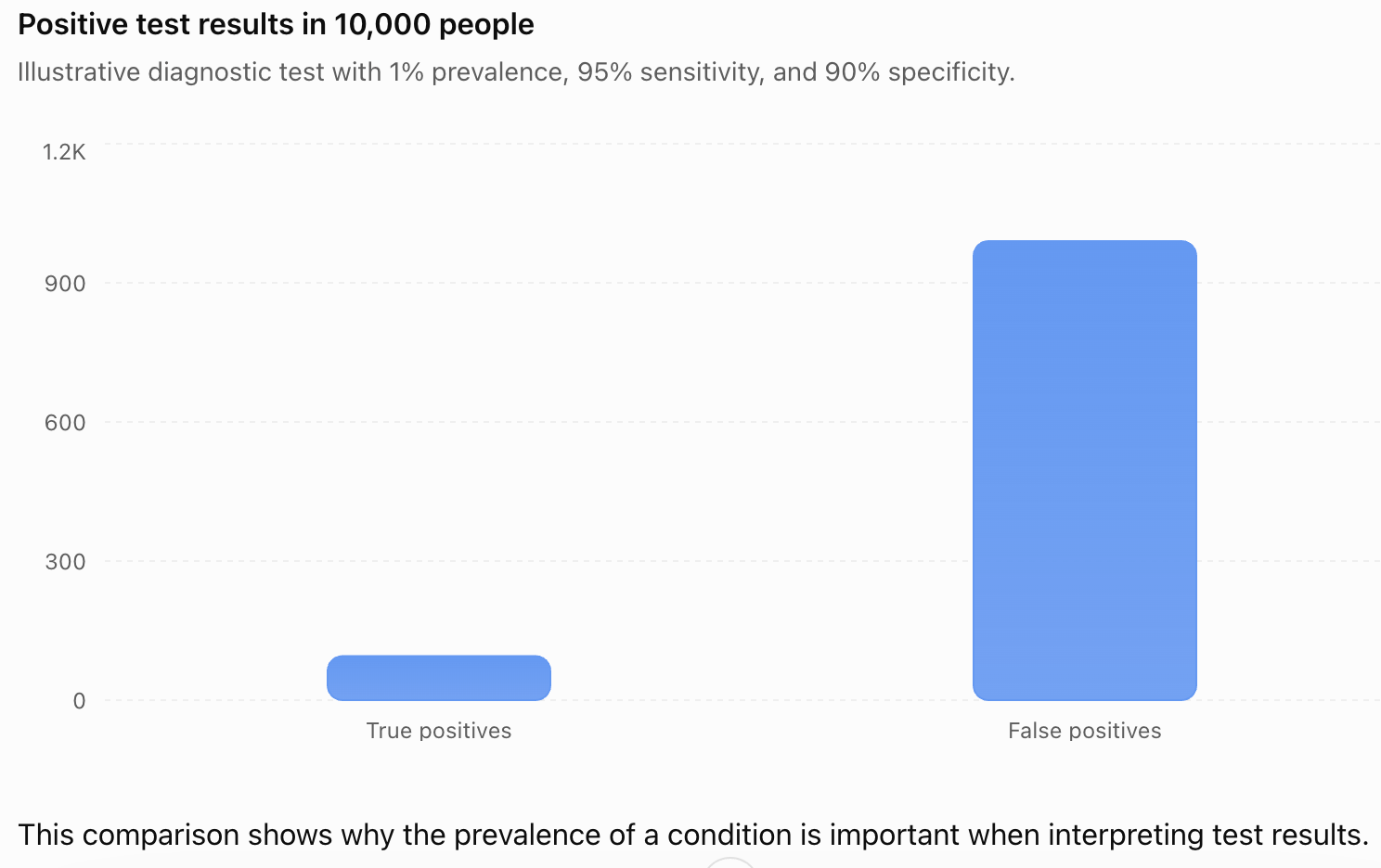
This comparison shows why the prevalence of a condition is important when interpreting test results.
Positive and Negative Predictive Values
Two additional measures are useful in diagnostic testing.
Positive Predictive Value
The positive predictive value (PPV) is the probability that a person has the condition given a positive test result.
PPV = P(condition | positive)
This is the posterior probability calculated using Bayes' Theorem.
Negative Predictive Value
The negative predictive value (NPV) is the probability that a person does not have the condition given a negative test result.
NPV = P(no condition | negative)
Using the previous example:
NPV = 8910/8915
NPV ≈ 0.9994 = 99.94%
Under this example's assumptions, a negative result is very likely to be correct.
Important Distinction
Sensitivity and specificity describe how a test performs among people whose actual condition is known.
Predictive values describe what a positive or negative result means for the person being tested.
Predictive values depend on the prevalence of the condition in the tested population.
How Prior Probability Affects Posterior Probability
Suppose a diagnostic test has:
-
Sensitivity = 95%
-
Specificity = 90%
The posterior probability after a positive result changes depending on how common the condition is.
|
Prevalence |
Probability of condition after positive test |
|---|---|
|
1% |
8.76% |
|
5% |
33.33% |
|
10% |
51.35% |
|
20% |
70.37% |
|
50% |
90.48% |
The test itself has not changed.
Only the prior probability has changed.
This demonstrates a central idea of Bayesian reasoning:
The same evidence can produce different posterior probabilities when the prior probabilities differ.
Probability Trees and Bayes' Theorem
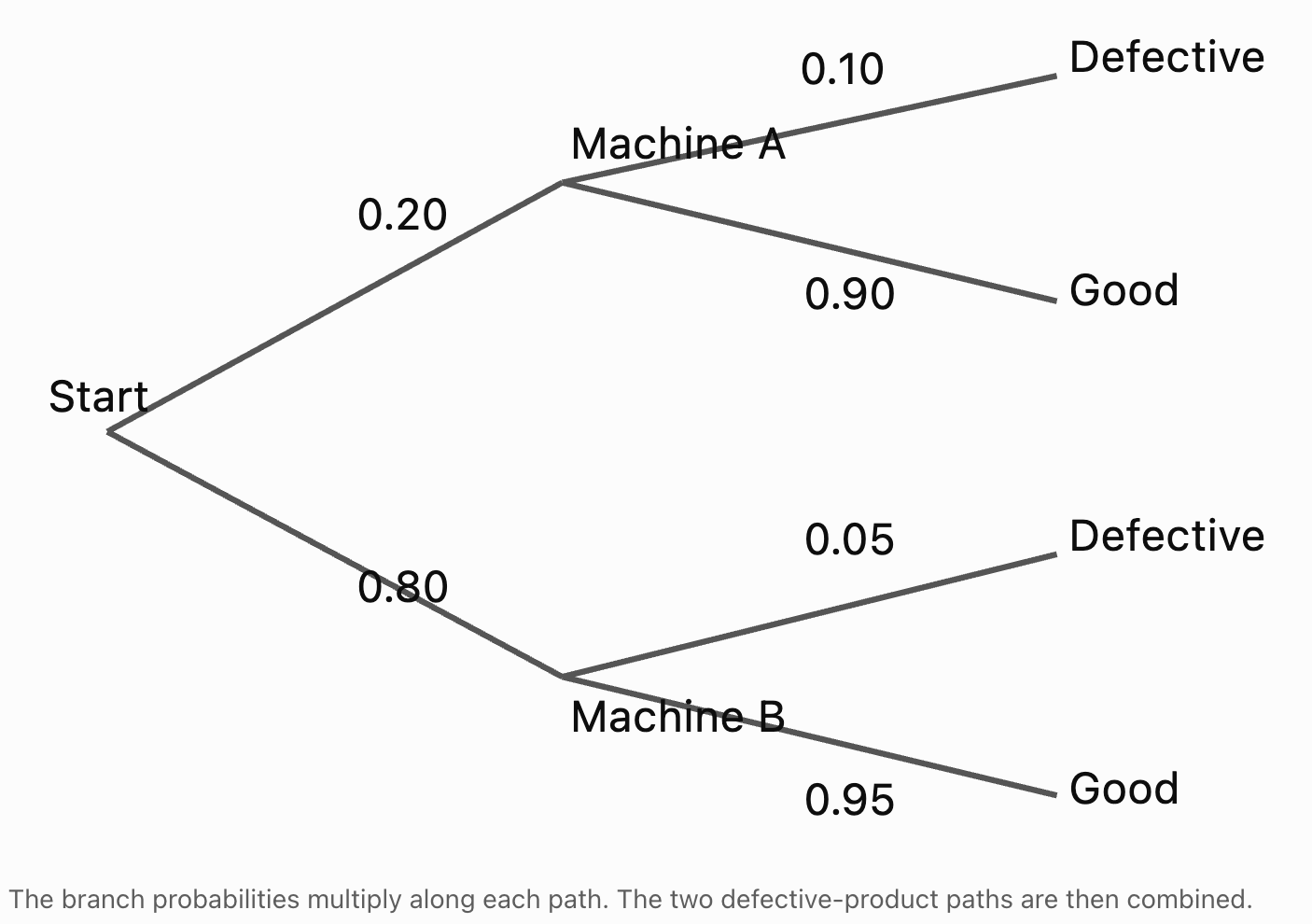
Probability trees provide another way to organize conditional probabilities.
Consider a simplified factory example.
-
20% of products come from Machine A.
-
80% come from Machine B.
-
Machine A produces defective products 10% of the time.
-
Machine B produces defective products 5% of the time.
We want to determine the probability that a defective product came from Machine A.
Step 1: Identify the Branches
Step 2: Calculate the Probability of a Defective Product from Each Machine
Machine A:
P(A and defective) = 0.20 × 0.10
= 0.02
Machine B:
P(B and defective) = 0.80 × 0.05
= 0.04
Step 3: Calculate the Total Probability of a Defect
P(defective) = 0.02 + 0.04
= 0.06
Step 4: Apply Bayes' Theorem
P(A | defective) = 0.02/0.06
P(A | defective) ≈ 0.3333
There is approximately a 33.33% probability that a defective product came from Machine A.
Although Machine A has a higher defect rate, Machine B produces more products overall.
Bayesian Reasoning in Everyday Life
Bayesian reasoning is not limited to formal probability calculations.
It describes a general process of updating beliefs when new information becomes available.
Weather Forecasting
A meteorologist may initially estimate a 30% probability of rain.
New satellite observations may provide evidence that increases or decreases this estimate.
The updated probability incorporates both the original forecast and the new evidence.
Email Spam Detection
An email system may estimate the probability that a message is spam.
Evidence might include:
-
Certain words or phrases.
-
Suspicious links.
-
Sender characteristics.
-
Previous patterns of unwanted messages.
The system can use probabilistic methods to update its estimate.
Scientific Investigations
Scientists often compare competing explanations for observed results.
As new experimental evidence becomes available, the relative support for different hypotheses may change.
Quality Control
Manufacturers can use inspection results to estimate the probability that a product is defective or that a particular machine caused a problem.


Bayesian Updating with Multiple Pieces of Evidence
Bayesian reasoning can be repeated as new evidence becomes available.
Suppose an initial probability is:
P(A) = 0.20
After observing evidence B, the probability is updated to:
P(A | B) = 0.60
If additional evidence C becomes available, the updated probability can be revised again:
P(A | B and C)
The previous posterior probability becomes part of the information used in the next update.
Sequential Updating
The process is:
Prior → Evidence → Posterior → New Evidence → New Posterior
This is useful in:
-
Medical investigations.
-
Scientific experiments.
-
Machine learning.
-
Weather forecasting.
-
Engineering diagnostics.
Important Limitation
Evidence must be combined carefully.
If two observations are related, treating them as independent can lead to incorrect probabilities.
For example, two medical tests may share the same sources of error.
Bayesian updating must account for such dependencies.
Bayesian Reasoning and Decision-Making
Bayes' Theorem can help people make decisions when information is incomplete.
However, probability alone does not determine the best decision.
Decision-makers must also consider the consequences of different outcomes.
For example, suppose a machine has a 10% probability of malfunctioning.
An inspection provides evidence that increases the estimated probability to 60%.
The company may decide to stop the machine for maintenance.
The decision depends on:
-
The updated probability of malfunction.
-
The cost of maintenance.
-
The cost of a possible failure.
-
Safety considerations.
-
Available alternatives.
Bayesian reasoning provides an improved estimate of uncertainty, while decision analysis considers what action should follow.
The Base-Rate Fallacy
A common error in probability reasoning is ignoring the initial frequency of an event.
This is called the base-rate fallacy.
Example
Suppose a rare condition affects only 1% of a population.
A test correctly identifies 99% of people with the condition.
Someone might conclude that a positive result means there is a 99% probability of having the condition.
This conclusion is not justified.
The probability after a positive result also depends on the false positive rate and the prevalence of the condition.
A highly sensitive test does not automatically have a high positive predictive value.
Avoiding the Base-Rate Fallacy
When interpreting evidence, always ask:
-
How common was the event before the evidence?
-
How likely is the evidence if the event is true?
-
How likely is the same evidence if the event is false?
These questions form the foundation of Bayesian reasoning.
Common Mistakes
Confusing P(A | B) with P(B | A)
Conditional probabilities are not generally interchangeable.
Ignoring the prior probability
Bayes' Theorem requires considering how likely an event was before the evidence.
Confusing sensitivity with positive predictive value
Sensitivity describes test performance among people with the condition. Positive predictive value describes the probability of the condition after a positive result.
Forgetting false positives
Evidence may occur even when the hypothesis is false.
Using the wrong denominator
The denominator in Bayes' Theorem is the overall probability of the observed evidence.
Forgetting the Law of Total Probability
Evidence can often arise through multiple mutually exclusive possibilities.
Assuming a positive test proves a condition is present
A positive result changes probability but does not establish certainty.
Ignoring the base rate
Rare events can remain relatively unlikely even after apparently strong evidence.
Treating dependent evidence as independent
Related observations may contain overlapping information.
Confusing probability with decision-making
An updated probability helps inform a decision, but consequences and costs must also be considered.
Key Terms
-
Bayes' Theorem: A mathematical rule for updating probabilities using new evidence.
-
Conditional Probability: The probability of an event occurring given that another event has occurred.
-
Prior Probability: The probability assigned to a hypothesis before considering new evidence.
-
Posterior Probability: The updated probability of a hypothesis after considering evidence.
-
Likelihood: The probability of observing particular evidence under a specified hypothesis.
-
Evidence Probability: The overall probability of observing the evidence.
-
Bayesian Updating: The process of revising probabilities when new information becomes available.
-
Law of Total Probability: A rule for calculating the probability of an event by combining probabilities across mutually exclusive cases.
-
Hypothesis: A proposed explanation or claim being evaluated.
-
Evidence: Information or observations used to evaluate a hypothesis.
-
Base Rate: The initial frequency or prevalence of an event in a population.
-
Base-Rate Fallacy: The error of ignoring prior probabilities when interpreting evidence.
-
Sensitivity: The probability that a diagnostic test is positive when the condition is present.
-
Specificity: The probability that a diagnostic test is negative when the condition is absent.
-
True Positive: A positive test result for someone who has the condition.
-
False Positive: A positive test result for someone who does not have the condition.
-
True Negative: A negative test result for someone who does not have the condition.
-
False Negative: A negative test result for someone who has the condition.
-
Positive Predictive Value: The probability that a condition is present given a positive test result.
-
Negative Predictive Value: The probability that a condition is absent given a negative test result.
-
Probability Tree: A branching diagram representing possible events and their probabilities.
-
Frequency Table: A table showing counts of outcomes in different categories.
-
Sequential Updating: Repeatedly revising probabilities as additional evidence becomes available.
-
Decision Analysis: The process of comparing possible actions using probabilities and consequences.
Key Takeaways
-
Bayes' Theorem allows probabilities to be updated when new evidence becomes available.
-
Conditional probability describes the likelihood of an event given that another event has occurred.
-
P(A | B) is not generally equal to P(B | A).
-
Bayes' Theorem connects prior probability, likelihood, evidence probability, and posterior probability.
-
The prior probability represents what was known before observing new evidence.
-
The posterior probability represents the updated probability after considering the evidence.
-
The Law of Total Probability is often used to calculate the denominator in Bayes' Theorem.
-
Diagnostic testing is an important application of Bayesian reasoning.
-
Sensitivity and specificity describe different aspects of test accuracy.
-
Positive predictive value depends on both test accuracy and condition prevalence.
-
A positive result does not necessarily mean that a condition is likely to be present.
-
Rare events can remain relatively unlikely after positive evidence because of the base-rate effect.
-
Frequency tables and probability trees can make Bayesian calculations easier to understand.
-
Bayesian updating can be repeated as new evidence becomes available.
-
Evidence must be combined carefully when observations are dependent.
-
Bayesian reasoning is useful in medicine, manufacturing, scientific research, weather forecasting, and information technology.
-
Updated probabilities support decision-making, but consequences and risks must also be considered.
Check Your Understanding
Recall and Understanding
-
State Bayes' Theorem and explain the meaning of each term.
-
Define prior probability and posterior probability.
-
Explain why P(A | B) is not generally equal to P(B | A).
-
Define sensitivity and specificity in diagnostic testing.
-
Explain the base-rate fallacy and why it can lead to incorrect conclusions.
Application
-
Suppose P(A) = 0.3, P(B | A) = 0.8, and P(B) = 0.5. Calculate P(A | B).
-
A factory produces 10% defective products. An inspection system flags 90% of defective products and 15% of non-defective products. Calculate the probability that a flagged product is actually defective.
-
A medical condition affects 2% of a population. A test has 95% sensitivity and 90% specificity. Calculate the probability that a person has the condition given a positive result.
-
A company uses two machines. Machine A produces 40% of products with a defect rate of 5%. Machine B produces 60% with a defect rate of 2%. Calculate the probability that a defective product came from Machine A.
-
A diagnostic test has sensitivity 98% and specificity 95%. Calculate the false positive and false negative rates.
Analysis and Challenge
-
A rare condition affects 0.5% of a population. A test has 99% sensitivity and 99% specificity. Calculate the probability that a person actually has the condition after a positive result.
-
Explain why the same diagnostic test can have different positive predictive values in populations with different condition prevalence.
-
A factory inspection system is improved so that its false positive rate decreases while sensitivity remains constant. Explain how this change affects the probability that a flagged product is actually defective.
-
A student receives two positive results from separate diagnostic tests. Explain why it may be incorrect to assume the tests are independent when updating the probability of a condition.
-
A weather forecast initially predicts a 20% probability of rain. New observations are more likely when rain is approaching than when conditions are dry. Explain how Bayes' Theorem could be used to update the forecast and identify the additional probabilities required.
Final Summary
Bayes' Theorem provides a mathematical framework for updating probabilities when new evidence becomes available.
By combining prior probabilities with the likelihood of observed evidence, we can calculate posterior probabilities and improve our understanding of uncertain situations.
Bayesian reasoning is especially important when interpreting diagnostic tests, evaluating scientific evidence, identifying manufacturing problems, and making decisions under uncertainty.
The central lesson is that evidence should never be interpreted in isolation. Its meaning depends on both how likely the evidence is under different explanations and how plausible those explanations were before the evidence was observed.
Understanding Bayes' Theorem helps students reason more accurately about probability, avoid common statistical errors, and make better-informed decisions in real-world situations.