3. Binomial Distribution

Binomial Distribution

Introduction to the Binomial Distribution

Many situations involve repeating an experiment and counting how many times a particular outcome occurs.

For example:

• How many heads will appear when a coin is tossed ten times?

• How many students will answer a multiple-choice question correctly?

• How many defective products will be found in a sample?

• How many basketball free throws will a player successfully make?

• How many seeds will germinate under controlled conditions?

These situations can often be modelled using the binomial distribution.

The binomial distribution is a discrete probability distribution that describes the number of successes in a fixed number of independent trials, where each trial has two possible outcomes and the probability of success remains constant.

It is one of the most widely used probability models in mathematics, science, statistics, and decision-making.

Understanding Binomial Experiments

A binomial experiment is a random experiment that satisfies four specific conditions.

A useful way to remember these conditions is BINS.

• B — Binary outcomes: Each trial has two possible outcomes, usually called success and failure.

• I — Independent trials: The outcome of one trial does not affect the probability of success in another.

• N — Number of trials fixed: The experiment contains a predetermined number of trials.

• S — Same probability: The probability of success remains constant for every trial.

All four conditions must be satisfied for the standard binomial model to apply.

Example: Tossing a Coin

Suppose a fair coin is tossed five times.

We define:

Success = obtaining heads

Failure = obtaining tails

Check the conditions:

Therefore, the experiment is binomial.

Example: Rolling a Die

Suppose a fair six-sided die is rolled eight times.

Let success mean rolling a 6.

Then:

p = 1/6

q = 5/6

Each roll is independent, and the probability of rolling a 6 remains constant.

This is also a binomial experiment.

A binomial trial does not require the two outcomes to be equally likely.

Identifying Experiments That Are Not Binomial

Not every experiment involving repeated observations is binomial.

Example: Rolling Until the First Six Appears

Suppose a die is rolled until the first 6 appears.

This is not a binomial experiment because the number of trials is not fixed.

Example: Drawing Cards Without Replacement

Suppose five cards are drawn from a standard deck without replacement.

Let success mean drawing a heart.

The probability of success changes after each card is drawn because the deck changes.

The trials are not independent, so the standard binomial model is not exact.

Example: Measuring Student Heights

Suppose the heights of ten students are recorded.

Height is a continuous measurement rather than a binary outcome.

This is not a binomial experiment as stated.

However, if each student is classified as either above or not above a particular height, the outcomes become binary. Independence and constant probability would still need to be justified.

Binomial Random Variables

A binomial random variable counts the number of successes in a binomial experiment.

It is commonly represented by X.

For example, if a fair coin is tossed four times:

X = number of heads

The possible values are:

X = 0, 1, 2, 3, 4

A binomial random variable is written as:

X ~ B(n, p)

where:

• n is the number of trials.

• p is the probability of success on each trial.

• X is the number of successes.

For example:

X ~ B(4, 0.5)

means that X counts successes in four independent trials, each with a success probability of 0.5.

Important Terminology

The probability of failure is commonly represented by q.

q = 1 − p

Therefore:

p + q = 1

If the probability of success is 0.7, the probability of failure is:

q = 1 − 0.7 = 0.3

The Binomial Probability Formula

The probability of obtaining exactly r successes in n independent trials is:

P(X = r) = C(n, r)pʳ(1 − p)^(n−r)

where:

• n = total number of trials

• r = number of successes

• p = probability of success

• 1 − p = probability of failure

• C(n, r) = number of ways to choose r successes from n trials

The combination formula is:

C(n, r) = n!/[r!(n − r)!]

The binomial formula combines counting and probability.

Why Does the Formula Work?

Consider three coin tosses.

We want exactly two heads.

One possible sequence is:

HHT

Its probability is:

0.5 × 0.5 × 0.5 = 0.125

However, there are three sequences containing exactly two heads:

• HHT

• HTH

• THH

The number of arrangements is:

C(3, 2) = 3

Therefore:

P(X = 2) = 3 × 0.125

P(X = 2) = 0.375

The combination term counts how many sequences contain the required number of successes.

The probability terms calculate the probability of each such sequence.

Calculating Binomial Probabilities

Worked Example: Exactly Three Heads

A fair coin is tossed five times.

Find the probability of obtaining exactly three heads.

Step 1: Identify the values.

n = 5

r = 3

p = 0.5

q = 0.5

Step 2: Substitute into the formula.

P(X = 3) = C(5, 3)(0.5)³(0.5)²

Step 3: Calculate the combination.

C(5, 3) = 10

Step 4: Calculate the probability.

P(X = 3) = 10 × 0.125 × 0.25

Final answer:

P(X = 3) = 0.3125

There is a 31.25% probability of obtaining exactly three heads.

Worked Example: Basketball Free Throws

A basketball player successfully makes 80% of free throws.

Assume each attempt is independent and the success probability remains constant.

The player takes five free throws.

What is the probability of making exactly four?

Step 1: Identify the values.

n = 5

r = 4

p = 0.8

q = 0.2

Step 2: Apply the formula.

P(X = 4) = C(5, 4)(0.8)⁴(0.2)¹

Step 3: Calculate.

C(5, 4) = 5

P(X = 4) = 5 × 0.4096 × 0.2

Final answer:

P(X = 4) = 0.4096

There is a 40.96% probability that the player makes exactly four of the five free throws.

Constructing a Binomial Probability Distribution

A binomial probability distribution shows the probability of every possible number of successes.

Consider three fair coin tosses.

Let:

X = number of heads

Then:

X ~ B(3, 0.5)

The possible values are:

0, 1, 2, 3

Calculate each probability.

P(X = 0) = C(3, 0)(0.5)⁰(0.5)³ = 0.125

P(X = 1) = C(3, 1)(0.5)¹(0.5)² = 0.375

P(X = 2) = C(3, 2)(0.5)²(0.5)¹ = 0.375

P(X = 3) = C(3, 3)(0.5)³(0.5)⁰ = 0.125

Probability Distribution Table

The probabilities add to 1, confirming that the distribution includes all possible outcomes.

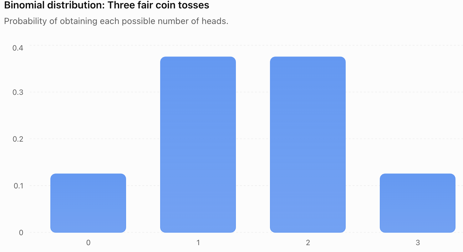
The distribution is symmetrical because p = 0.5.

Obtaining one or two heads is more likely than obtaining zero or three heads.

Exploring How Binomial Distributions Change

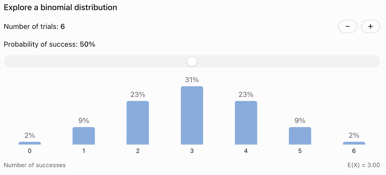
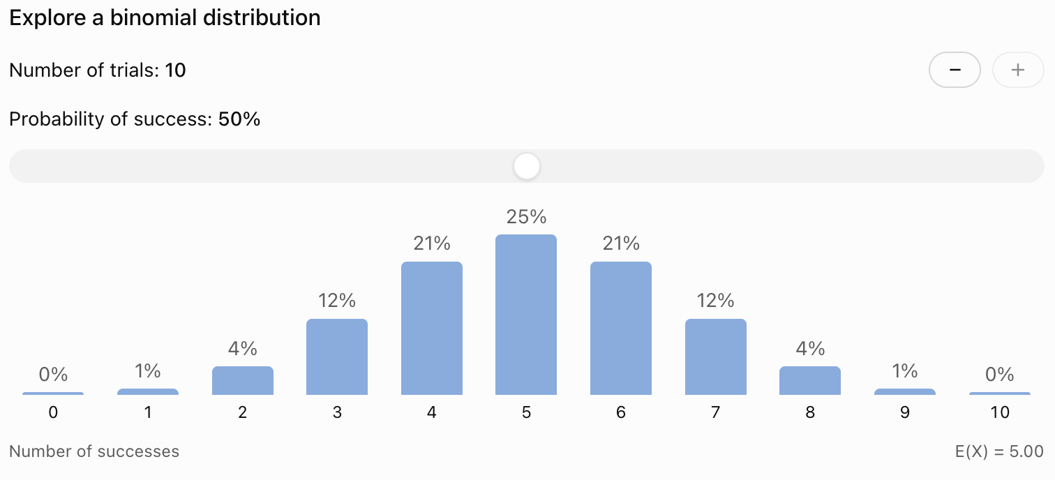
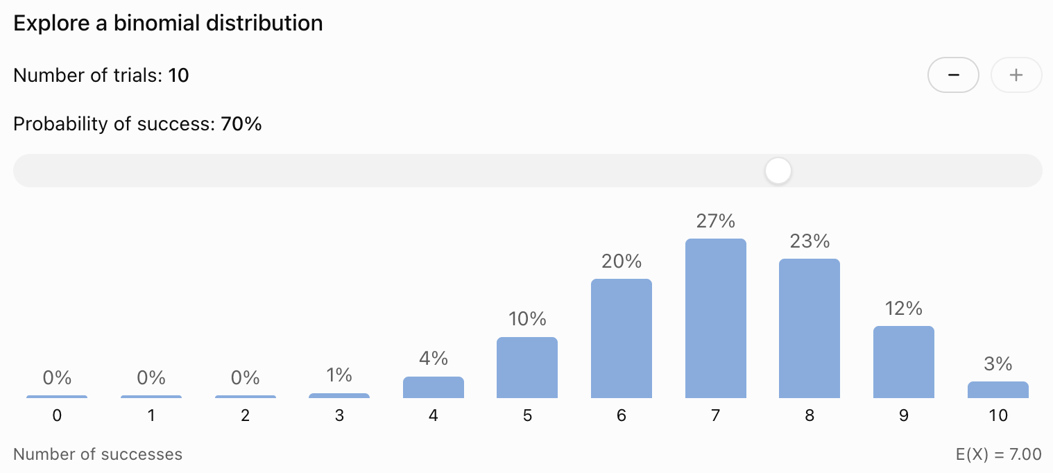
The shape of a binomial distribution depends on:

• The number of trials, n.

• The probability of success, p.

When p = 0.5, the distribution is symmetrical.

When p is small, most of the probability is concentrated toward lower numbers of successes.

When p is large, most of the probability is concentrated toward higher numbers of successes.

Calculating Probabilities for More Than One Outcome

Binomial problems often ask for probabilities involving several possible numbers of successes.

Common expressions include:

• Exactly r successes: P(X = r)

• At most r successes: P(X ≤ r)

• Fewer than r successes: P(X < r)

• At least r successes: P(X ≥ r)

• More than r successes: P(X > r)

It is important to interpret these expressions correctly.

At Most

"At most three successes" means:

X ≤ 3

This includes:

0, 1, 2, or 3 successes.

At Least

"At least three successes" means:

X ≥ 3

This includes:

3, 4, 5, ... up to n successes.

More Than

"More than three successes" means:

X > 3

This begins at four successes.

Fewer Than

"Fewer than three successes" means:

X < 3

This includes zero, one, or two successes.

Worked Example: At Most Two Successes

A fair coin is tossed four times.

Find the probability of obtaining at most two heads.

Let:

X ~ B(4, 0.5)

We want:

P(X ≤ 2)

Therefore:

P(X ≤ 2) = P(X = 0) + P(X = 1) + P(X = 2)

Calculate:

P(X = 0) = 1/16

P(X = 1) = 4/16

P(X = 2) = 6/16

Add:

P(X ≤ 2) = 1/16 + 4/16 + 6/16

= 11/16

P(X ≤ 2) = 0.6875

There is a 68.75% probability of obtaining at most two heads.

Complementary Probability

Sometimes it is easier to calculate the probability of the opposite event and subtract it from 1.

The complementary probability rule is:

P(A) = 1 − P(not A)

This is particularly useful for binomial problems involving "at least one" or "at least r."

Worked Example: At Least One Success

A machine produces defective items with probability 0.05.

Assume defects occur independently.

Five items are selected.

What is the probability that at least one is defective?

Let:

X = number of defective items

n = 5

p = 0.05

We want:

P(X ≥ 1)

Instead of calculating five separate probabilities, use the complement.

P(X ≥ 1) = 1 − P(X = 0)

P(X = 0) = C(5, 0)(0.05)⁰(0.95)⁵

= 0.95⁵

≈ 0.7738

Therefore:

P(X ≥ 1) = 1 − 0.7738

P(X ≥ 1) ≈ 0.2262

There is approximately a 22.62% probability that at least one item is defective.

Worked Example: At Least Four Successes

A student answers five independent true-or-false questions by guessing.

Each question has a 50% probability of being answered correctly.

Find the probability of answering at least four correctly.

Let:

X ~ B(5, 0.5)

We want:

P(X ≥ 4)

This includes four or five correct answers.

P(X ≥ 4) = P(X = 4) + P(X = 5)

P(X = 4) = C(5, 4)(0.5)⁴(0.5)¹

= 5/32

P(X = 5) = C(5, 5)(0.5)⁵

= 1/32

Therefore:

P(X ≥ 4) = 6/32

P(X ≥ 4) = 0.1875

There is an 18.75% probability of answering at least four questions correctly by guessing.

Expected Value of a Binomial Distribution

The expected value represents the average number of successes that would be obtained over many repetitions of the experiment.

For a binomial random variable:

E(X) = np

where:

• n is the number of trials.

• p is the probability of success.

Worked Example: Basketball Shots

A player has a 70% probability of making each basketball shot.

The player attempts 20 shots.

Find the expected number of successful shots.

n = 20

p = 0.7

E(X) = np

= 20 × 0.7

E(X) = 14

The expected number of successful shots is 14.

This does not mean the player will make exactly 14 shots every time.

It means that over many sets of 20 attempts, the average number of successful shots would approach 14, assuming the model is accurate.

Variance of a Binomial Distribution

The variance measures how widely the number of successes tends to vary around the expected value.

For a binomial random variable:

Var(X) = np(1 − p)

or:

Var(X) = npq

where:

q = 1 − p

Worked Example: Variance of Basketball Shots

Using the previous example:

n = 20

p = 0.7

q = 0.3

Var(X) = 20 × 0.7 × 0.3

Var(X) = 4.2

The variance is 4.2 successes².

Standard Deviation of a Binomial Distribution

The standard deviation is the positive square root of the variance.

σ = √[np(1 − p)]

For the basketball example:

σ = √4.2

σ ≈ 2.05

Interpretation

The expected number of successful shots is 14.

The standard deviation is approximately 2.05 shots.

This describes the scale of variation around the expected number of successes.

A standard deviation is not a strict boundary. Results can be more than one standard deviation away from the mean.

Comparing Binomial Distributions

Consider two binomial experiments.

Experiment A

n = 20

p = 0.5

Expected value:

E(X) = 20 × 0.5 = 10

Variance:

Var(X) = 20 × 0.5 × 0.5 = 5

Standard deviation:

σ = √5 ≈ 2.24

Experiment B

n = 20

p = 0.9

Expected value:

E(X) = 20 × 0.9 = 18

Variance:

Var(X) = 20 × 0.9 × 0.1 = 1.8

Standard deviation:

σ = √1.8 ≈ 1.34

Experiment B has a higher expected number of successes but a smaller standard deviation.

When the probability of success is close to 0 or 1, the binomial distribution tends to be less spread out than when p is near 0.5, for the same n.

Shape of the Binomial Distribution

The shape of a binomial distribution depends on n and p.

When p = 0.5

The distribution is symmetrical.

Successes and failures are equally likely.

When p < 0.5

The distribution is generally right-skewed, with more probability concentrated toward smaller numbers of successes.

When p > 0.5

The distribution is generally left-skewed, with more probability concentrated toward larger numbers of successes.

When n Increases

As the number of trials increases, the number of possible success counts increases.

For sufficiently large n, when neither np nor n(1 − p) is too small, the binomial distribution can be approximated by a normal distribution.

This is useful for calculations involving large numbers of trials.

Using Technology to Calculate Binomial Probabilities

Scientific calculators, spreadsheets, and statistical software can calculate binomial probabilities efficiently.

Common calculator functions include:

• binompdf(n, p, r): Calculates the probability of exactly r successes.

• binomcdf(n, p, r): Calculates the probability of at most r successes.

Function names vary by calculator or software.

Example: Exactly Three Successes

Suppose:

n = 10

p = 0.4

r = 3

A calculator may use:

binompdf(10, 0.4, 3)

The result is approximately:

0.2150

Example: At Most Three Successes

Using the same distribution:

binomcdf(10, 0.4, 3)

The result is approximately:

0.3823

Technology is especially useful when the number of trials is large.

However, students should still understand the formula and the meaning of the results.

Practical Application: Quality Control

A factory produces electronic components.

The probability that a component is defective is 0.03.

Assume defects occur independently and the probability remains constant.

A quality-control inspector examines 20 components.

Let:

X = number of defective components

Then:

X ~ B(20, 0.03)

Expected Number of Defective Components

E(X) = np

= 20 × 0.03

E(X) = 0.6

The expected number of defective components is 0.6 per sample of 20.

Variance

Var(X) = 20 × 0.03 × 0.97

Var(X) = 0.582

Standard Deviation

σ = √0.582

σ ≈ 0.763

Probability of No Defective Components

P(X = 0) = C(20, 0)(0.03)⁰(0.97)²⁰

= 0.97²⁰

P(X = 0) ≈ 0.5438

There is approximately a 54.38% probability that all 20 components are non-defective.

Interpretation

Although the expected number of defects is less than one, some samples may contain several defects.

The binomial distribution allows the company to estimate the likelihood of different outcomes and make quality-control decisions.

Practical Application: Medical Testing

Suppose a screening test has a 90% probability of correctly identifying a particular condition in a person who has it.

Assume ten tests are conducted on different people who all have the condition, and that the test results are independent with the same sensitivity.

Let:

X = number of correctly identified cases

Then:

X ~ B(10, 0.9)

Expected Number of Correct Results

E(X) = 10 × 0.9

E(X) = 9

Probability of Exactly Nine Correct Results

P(X = 9) = C(10, 9)(0.9)⁹(0.1)¹

≈ 0.3874

P(X = 9) ≈ 0.3874

There is approximately a 38.74% probability that exactly nine of the ten cases are correctly identified.

Important Limitation

Real medical testing situations may involve different probabilities, dependent observations, or other complications.

A binomial model is appropriate only when its assumptions are reasonable.

Practical Application: Seed Germination

A scientist investigates the germination of seeds.

Under controlled conditions, each seed has an estimated 80% probability of germinating.

Assume the germination outcomes are independent.

The scientist plants 15 seeds.

Let:

X = number of seeds that germinate

Then:

X ~ B(15, 0.8)

Expected Value

E(X) = 15 × 0.8

E(X) = 12

Variance

Var(X) = 15 × 0.8 × 0.2

Var(X) = 2.4

Standard Deviation

σ = √2.4

σ ≈ 1.55

Interpretation

The scientist expects approximately 12 seeds to germinate.

However, the actual number may vary from one experiment to another.

The model helps predict likely outcomes and compare results from repeated investigations.

Evaluating Binomial Models

A mathematical model is useful only when its assumptions reasonably match the real situation.

Before applying a binomial distribution, consider the following questions.

Are There Exactly Two Outcomes?

Each trial must be classified as success or failure.

For example, a product may be classified as defective or non-defective.

Are the Trials Independent?

One trial must not affect the outcome probabilities of another.

This assumption may fail when sampling without replacement from a small population.

Is the Number of Trials Fixed?

The total number of trials must be determined before the experiment begins.

Is the Probability Constant?

The probability of success must remain the same across all trials.

For example, a basketball player's probability of making a shot may change because of fatigue, distance, or defensive pressure.

Is the Model Realistic?

Even if the conditions appear approximately satisfied, real-world factors may influence the results.

Mathematical models simplify reality, so their limitations should be considered when interpreting conclusions.

A Strategy for Solving Binomial Problems

When solving a binomial probability problem, use the following method.

Identify the experiment.

Determine what counts as one trial and what is considered a success.

Check the binomial conditions.

Confirm that the experiment satisfies BINS.

Define the random variable.

For example:

X = number of successful attempts

Identify n and p.

Determine the number of trials and the probability of success.

Interpret the question carefully.

Decide whether the question asks for exactly, at most, at least, more than, or fewer than a particular number of successes.

Choose the correct method.

Use the binomial probability formula, add relevant probabilities, or apply complementary counting.

Calculate and interpret the result.

Express the probability as a decimal, fraction, or percentage, and explain its meaning in context.

Common Mistakes

Using the binomial formula when the conditions are not satisfied

Always check that the trials are independent, the number of trials is fixed, and the success probability is constant.

Confusing n and r

n represents the total number of trials, while r represents the number of successes.

Using the wrong probability

The probability p must correspond to the event defined as success.

Forgetting the combination term

C(n, r) counts the number of different sequences containing r successes.

Confusing exactly, at least, and at most

These expressions represent different sets of outcomes.

Forgetting complementary probability

Problems involving "at least one" are often easier to solve using 1 − P(X = 0).

Assuming the expected value must be a possible outcome

An expected value of 0.6 defective components is mathematically valid.

Confusing variance with standard deviation

Standard deviation is the square root of variance.

Assuming every binomial distribution is symmetrical

Symmetry occurs when p = 0.5.

Ignoring real-world assumptions

A binomial model may not accurately describe situations involving dependence or changing probabilities.

Key Terms

• Binomial Distribution: A discrete probability distribution describing the number of successes in a fixed number of independent trials with constant success probability.

• Binomial Experiment: A random experiment satisfying the four binomial conditions.

• Trial: One repetition of a random experiment.

• Success: The outcome of interest in a binomial experiment.

• Failure: The alternative outcome to success.

• Independent Trials: Trials in which one outcome does not affect the probabilities of other outcomes.

• Fixed Number of Trials: A predetermined number of repetitions.

• Constant Probability: A success probability that remains unchanged between trials.

• Binomial Random Variable: A variable counting the number of successes in a binomial experiment.

• Probability Distribution: A description of the probabilities associated with possible values of a random variable.

• Combination: A selection of objects where order does not matter.

• Binomial Coefficient: The value C(n, r), representing the number of ways to choose r objects from n.

• Complementary Probability: The probability that an event does not occur.

• Cumulative Probability: The probability of obtaining a value at or below a specified value.

• Expected Value: The long-run average number of successes.

• Variance: A measure of how widely outcomes are spread around the expected value.

• Standard Deviation: The positive square root of variance.

• Symmetrical Distribution: A distribution whose probabilities mirror each other around its centre.

• Skewed Distribution: A distribution with greater spread or a longer tail on one side.

• Normal Approximation: A method of approximating a binomial distribution using a normal distribution when appropriate conditions are satisfied.

• Mathematical Model: A mathematical representation of a real-world situation.

• Probability of Success: The probability p that a trial produces the outcome of interest.

• Probability of Failure: The probability q = 1 − p that a trial does not produce the outcome of interest.

Key Takeaways

• The binomial distribution models the number of successes in repeated independent trials.

• A binomial experiment must satisfy the BINS conditions: Binary outcomes, Independent trials, fixed Number of trials, and Same probability.

• The binomial probability formula is P(X = r) = C(n, r)pʳ(1 − p)^(n−r).

• The combination term counts the number of ways successes can be arranged among the trials.

• The probability of failure is q = 1 − p.

• Binomial probabilities can describe exactly, at most, at least, more than, or fewer than a specified number of successes.

• Complementary probability is especially useful for questions involving at least one success.

• The expected value of a binomial random variable is E(X) = np.

• The variance is Var(X) = np(1 − p).

• The standard deviation is σ = √[np(1 − p)].

• The shape of a binomial distribution depends on the number of trials and the probability of success.

• Binomial distributions are symmetrical when p = 0.5.

• For a fixed n, the variance is greatest when p = 0.5.

• Technology can simplify calculations involving large numbers of trials.

• Binomial models are useful in sports, quality control, genetics, medical testing, education, and scientific experiments.

• Binomial models should be evaluated carefully to ensure their assumptions are appropriate.

Check Your Understanding

Recall and Understanding

1. Define a binomial experiment and state its four required conditions.

2. Explain the difference between success and failure in a binomial experiment.

3. State the binomial probability formula and explain the meaning of n, r, and p.

4. Explain why combinations are used in binomial probability calculations.

5. Describe how changing p affects the shape of a binomial distribution.

Application

6. A fair coin is tossed five times. Calculate the probability of obtaining exactly three heads.

7. A basketball player makes 75% of free throws. Calculate the probability of making exactly four out of six attempts, assuming independent attempts.

8. A fair die is rolled eight times. Calculate the probability of obtaining exactly two sixes.

9. A machine produces defective items with probability 0.04. Find the probability that none of ten independently produced items is defective.

10. A binomial random variable has n = 20 and p = 0.3. Calculate its expected value, variance, and standard deviation.

Analysis and Challenge

11. A student guesses on six independent true-or-false questions. Calculate the probability of answering at least five correctly.

12. A factory produces components with a 2% defect probability. Calculate the probability that at least one of 15 independently produced components is defective.

13. A basketball player makes 80% of free throws. Compare the expected number of successful shots and standard deviation for 10 attempts and 20 attempts.

14. Explain why drawing five cards from a deck without replacement does not satisfy the standard binomial conditions. Suggest a modification that would make the experiment binomial.

15. A scientist estimates that each seed has a 70% probability of germinating independently. For 12 seeds, calculate the probability that at least ten germinate, and explain how the result could be used in planning an experiment.

Final Summary

The binomial distribution provides a systematic method for calculating probabilities involving repeated experiments with two possible outcomes.

By identifying the binomial conditions, defining the random variable, and applying the binomial probability formula, students can calculate the likelihood of different numbers of successes.

Expected value, variance, and standard deviation provide additional information about the centre and spread of the distribution.

The binomial distribution is especially useful in practical situations involving repeated independent events, such as coin tosses, sports performance, quality control, and scientific investigations.

Understanding the assumptions and limitations of binomial models is essential for interpreting results accurately and making informed decisions.