Foundations of Probability

5. Tree Diagrams and Tables

Learning outcomes
  • I can construct probability tree diagrams.
  • I can interpret probability tables.
  • I can calculate probabilities using trees.
  • I can solve sequential probability problems.
  • I can communicate probability reasoning clearly.

Tree Diagrams and Tables

Probability problems become more challenging when an experiment has several stages or when information is divided into different groups. Two of the most useful tools for organizing these situations are probability tree diagrams and probability tables.

A tree diagram shows how an experiment develops step by step. A probability table organizes information into rows and columns so that relationships between events can be seen clearly.

These representations help us answer questions such as:

  • What is the probability that two events both occur?
  • What is the probability of one outcome followed by another?
  • How does an earlier result affect a later probability?
  • What is the probability of one of several possible sequences?
  • How can information from a survey or experiment be organized systematically?

The mathematics behind these methods is based largely on two ideas:

Along a path → multiply probabilities

Between alternative successful paths → add probabilities

https://images.openai.com/static-rsc-4/hc8rJHS9R330_IMhiBxMKWtyoVDijijJjhHpGeoMhDZe0Km7RPnlckWdJy8m9NPozzJ7TmDh0hT7DA-Kf_otWyPQ6oBDZfkH0fZeIJSosfuKXub0XgQ4FSjQnOBsZpk6KnCnfn8iziHb7cNEuvk06i-wwdRmJRBcqk8-ALfMan_ptuygpzlvG7XgswhwOdX0?purpose=fullsize
 
https://images.openai.com/static-rsc-4/Za6ll4eQLnUYlkMbo5gtuao1YYKhvSxgatk7vaA--BV-P9iIgeHTi9TRt19-trTimIkSzQhNjjgJwpZX1pize49_GiU4NMrArKOuG41S04rv2J7gGrM2rIqFRZCOlf4GkJKifUuV2mK7m4BcvohdQaVUz7zfUijD_6kWYEYKd2L0FibtYjYIs-H2y9y06YOe?purpose=fullsize
 
https://images.openai.com/static-rsc-4/yhIi0xFgZlpRl63FiFmXs3yNZEA_mzIfLsB_8GJsTlkL1OMooSgA_Nk_9wDnokEaW2blFmc7g_M6kRT0F4bhjpEZyXlunZb4kYztXx1H12MDxp_qYgMjIY9aozvgbL2K1WMwGQJaHPZHK70z6eiJAfRuk5v5L8lmKp0r9MF19K4M0b58VqOrDx6wjBgaHhcX?purpose=fullsize
 
6

Why Use Probability Trees?

A probability tree diagram shows the possible outcomes of a sequence of events.

Each branch represents one possible outcome.

Suppose a fair coin is tossed twice.

The first toss has two possibilities:

H or T

From each of these outcomes, the second toss again has:

H or T

The final possible sequences are:

HH, HT, TH, TT

A tree diagram makes these possibilities easy to see.


The Structure of a Tree Diagram

A probability tree normally contains:

  • a starting point
  • branches representing possible outcomes
  • probabilities written on the branches
  • additional branches for later stages
  • final outcomes at the ends
  • sometimes the probability of each complete path

For a two-stage experiment:

Start → First Event → Second Event → Final Outcome

Each route from the beginning to the end represents one possible sequence.


Branch Probabilities

Probabilities are written on the branches.

For a fair coin:

P(H) = 1/2

P(T) = 1/2

The probabilities leaving the same point must add to:

1

because one of the possible outcomes must occur.

Therefore:

1/2 + 1/2 = 1

If a spinner has:

P(red) = 0.3

P(blue) = 0.5

P(green) = 0.2

then:

0.3 + 0.5 + 0.2 = 1

This is a useful way to check whether a probability tree has been constructed correctly.


Multiply Along a Path

To calculate the probability of a particular sequence, multiply the probabilities along its branches.

Suppose a fair coin is tossed twice.

Find:

P(HH)

First toss heads:

1/2

Second toss heads:

1/2

Therefore:

P(HH)

= 1/2 × 1/2

= 1/4

Similarly:

P(HT)

= 1/2 × 1/2

= 1/4

The multiplication occurs because we are asking for:

heads AND heads

https://images.openai.com/static-rsc-4/HRkPGx8_GmRe0Cv530TRiHdtnfoEhqW1ITmCQHViOsKrZcHNo4sXNdHrxjcrk4ltybq8f10VWh0dn2XMdttYDKZ-DxV_p61E2VUn4lpVTEpPUSQCsApxewsaJyb2YnZnfMhjBItq-yrz601pA23N2FaOsHOmIU6L1KldhlOJIxkNKXuC-pBGeF9o8phakMN5?purpose=fullsize
 
https://images.openai.com/static-rsc-4/6d-3o3QzGaUzrj9hPqsHWFzSlIolujhVL9AR1lshsZCEhe0S9IHr_LEGg511KPGdXJRYOrecSZ3nr6RlKGdns1fpk-R-s6c6ia8WbSQm5vM3VLZYrdu2-zIrokk0ouFldm0g1dTM9Qj7lZzxvNCC3Yio6ZdSPUHEDutiIXzfgqI6neq50cKOFHizMB31pnJ5?purpose=fullsize
 
https://images.openai.com/static-rsc-4/s7udaTt2M9Zt11854z2b_ciplnn2sBBx4tx3nLnzJqbPGYLL4PaiIuu1zYQTWvuzp5Vl_XRVwLIzDW6sKJjKaQuV9RrKNN_GmqRtwaZmpgb8N-x7dbKseVyUtnCWqfbcGVhmpTBheda34jUhxRLh8OLbFRrjOmbVoAFy4NMstT8UgFKZtSufv5ddKz95nxpI?purpose=fullsize
 

Add Alternative Paths

Sometimes an event can happen through several different paths.

Suppose we toss a fair coin twice and want:

exactly one head

This can occur as:

HT

or:

TH

Each path has probability:

1/2 × 1/2 = 1/4

Therefore:

P(exactly one head)

= P(HT) + P(TH)

= 1/4 + 1/4

= 1/2

This gives the important tree-diagram rule:

Multiply along branches.

Add the probabilities of appropriate alternative paths.


Independent Events on a Tree

Events are independent when one event does not change the probability of another.

Suppose we:

  1. toss a fair coin
  2. roll a fair six-sided die

The coin result does not affect the die.

So from either H or T, the probabilities for the die remain:

1/6, 1/6, 1/6, 1/6, 1/6, 1/6

For example:

P(H and 6)

= 1/2 × 1/6

= 1/12

When events are independent, the probabilities at later stages remain unchanged by earlier outcomes.


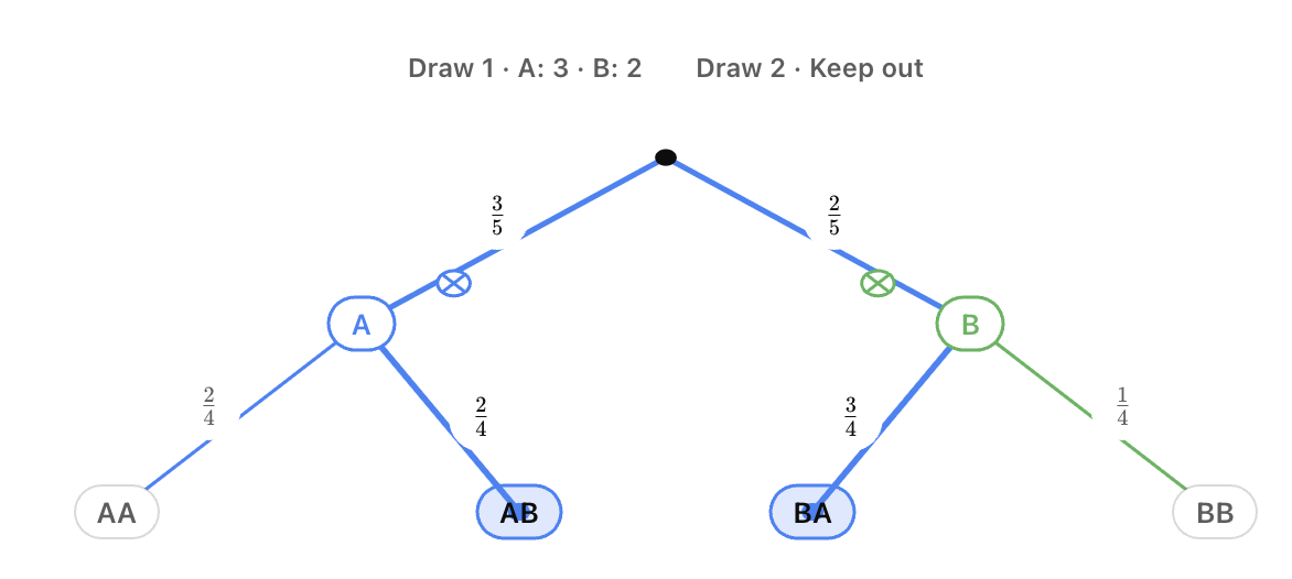
Dependent Events on a Tree

Events are dependent when an earlier outcome changes a later probability.

This often happens when objects are selected without replacement.

Suppose a bag contains:

3 red marbles

2 blue marbles

Two marbles are selected without replacement.

On the first draw:

P(R) = 3/5

P(B) = 2/5

If the first marble is red, the bag now contains:

2 red

2 blue

Therefore:

P(R second | R first) = 2/4

P(B second | R first) = 2/4

But if the first marble is blue, the bag contains:

3 red

1 blue

Therefore:

P(R second | B first) = 3/4

P(B second | B first) = 1/4

The second-stage probabilities depend on what happened first.

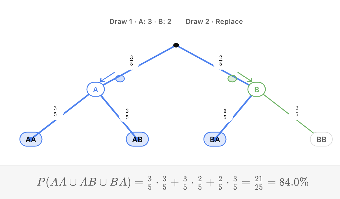
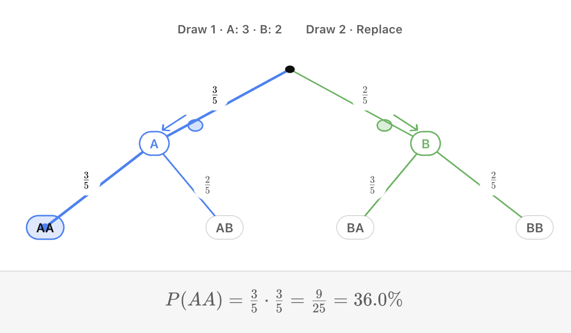
Here you can explore exactly how those branches change when sampling with or without replacement:
Worked Example: Two Red Marbles

Using the bag:

3 red

2 blue

Find the probability of drawing two red marbles without replacement.

Follow the RR path:

First red:

3/5

Second red given first red:

2/4

Therefore:

P(RR)

= 3/5 × 2/4

= 6/20

= 3/10


Worked Example: One of Each Colour

Using the same bag, find the probability of drawing one red and one blue.

There are two possible sequences:

RB

or:

BR

Red then Blue

P(RB)

= 3/5 × 2/4

= 6/20

= 3/10

Blue then Red

P(BR)

= 2/5 × 3/4

= 6/20

= 3/10

Now add the two paths:

P(one of each)

= 3/10 + 3/10

= 3/5


With Replacement

Now suppose the first marble is returned to the bag before the second draw.

The bag always contains:

3 red

2 blue

Therefore, on both draws:

P(R) = 3/5

P(B) = 2/5

The probabilities do not change.

For example:

P(RR)

= 3/5 × 3/5

= 9/25

Replacement often makes repeated selections independent.


Without Replacement vs With Replacement

This distinction is extremely important.

With Replacement

The selected object is returned.

The total number of objects returns to its original value.

The probabilities generally remain the same.

Without Replacement

The selected object is not returned.

The total decreases.

The composition may change.

Later probabilities therefore depend on earlier results.

https://images.openai.com/static-rsc-4/H0Q_Suf2L6U38YJVB6IoNvM_r0vaGGV1uHys2rtROqxgEI11SZVuNVTaD-NoYaeOrItja0cMTxivFADAuhlsklGfXtfi2t2fyVXDY7dkTS7g3tNm023z4XhV1NDZBIxE2_J6Nlk4p8RvleaBI4aNKszgha-Obk3r06nHiyCexH2BvSgKrYvodHnuja45Km-3?purpose=fullsize
 
https://images.openai.com/static-rsc-4/bJA_Hk-17BbtrWY5oxPIbdklB7_I7dUD9h8iScnF2zVi6NgpFEszvi9WYzcDwHeldXDxIPP9FAw3mYBRfGm4sz2RDxOWqKX8Rsk7MD57EnNfrhZmP90uvd9O0f9Blxk18f5drbsQVnEv-vPZhcmqynlp6OxEpYQlsxMGNAxY-lWpcMPEE0c85SpMU2q93fsa?purpose=fullsize
 
https://images.openai.com/static-rsc-4/vOVPKKOuJOC6nNald3KoIAXHKxGAjatd8gJo__2Ck-2ftrq7pT0aKLLEcjhsRWqswrt_VnZeomRyJc4v27C5GBdi7gKOfhMNAskBCkVs9mY5KDuoQ8jh-xgox2JgE5bRJu2hywaM-YLmgBHuOOWTb4-Gb8sPiMQwSuNKJLYXf_OXqRbipyw3VViumT_GeZS9?purpose=fullsize
 
5

A Three-Stage Tree

Tree diagrams can contain more than two stages.

Suppose a fair coin is tossed three times.

There are:

2 × 2 × 2 = 8

possible final outcomes:

HHH
HHT
HTH
HTT
THH
THT
TTH
TTT

Each individual path has probability:

1/2 × 1/2 × 1/2

= 1/8

A larger tree helps ensure that no possible sequence is forgotten.


Worked Example: Exactly Two Heads

For three fair coin tosses, exactly two heads can occur as:

HHT

HTH

THH

Each has probability:

1/8

Therefore:

P(exactly two heads)

= 1/8 + 1/8 + 1/8

= 3/8

Again:

multiply along each path

then:

add the successful paths


At Least One Event

Tree diagrams can also help with at least one problems.

Suppose a coin is tossed three times.

We want:

P(at least one head)

We could add all paths containing a head.

But there are seven such paths.

It is easier to use the complement.

The only outcome with no heads is:

TTT

P(TTT)

= 1/2 × 1/2 × 1/2

= 1/8

Therefore:

P(at least one H)

= 1 − 1/8

= 7/8

Sometimes a tree helps us recognize when the complement is the easier method.


Unequal Branch Probabilities

Tree diagrams are not limited to equally likely outcomes.

Suppose:

P(rain) = 0.30

P(no rain) = 0.70

If it rains:

P(bus late | rain) = 0.50

P(bus on time | rain) = 0.50

If it does not rain:

P(bus late | no rain) = 0.10

P(bus on time | no rain) = 0.90

The probabilities at each branching point still add to 1.


Worked Example: Bus Is Late

The bus can be late through two paths:

rain AND late

or:

no rain AND late

Rain and late:

0.30 × 0.50

= 0.15

No rain and late:

0.70 × 0.10

= 0.07

Therefore:

P(late)

= 0.15 + 0.07

= 0.22

So the probability that the bus is late is:

22%

This problem uses both multiplication and addition.


Interpreting a Tree Backwards

Sometimes we know the final outcome and want to determine something about an earlier event.

Using the previous example:

P(rain and late) = 0.15

P(late) = 0.22

Suppose we know that the bus was late.

What is the probability that it rained?

P(rain | late)

= 0.15/0.22

≈ 0.682

So approximately:

68.2%

This connects probability trees with conditional probability.


Tree Diagrams in Real Situations

Probability trees can represent:

  • medical test results
  • manufacturing defects
  • weather conditions
  • sporting outcomes
  • genetics
  • insurance risks
  • quality control
  • repeated selections
  • customer behaviour
  • reliability of systems

The branches do not have to represent coins, dice, or marbles.

They can represent any sequence of uncertain events.

https://images.openai.com/static-rsc-4/mQ9ChK-_54CtZODdTQe3dB5Yb-YYy_xM7FLcRYxNyDxe8nLWYEWkqgSdQCvvjPqk33FGkjt08xgfi-LcypCFz1Kdd1K6HnoC-ehZwd0FAM0p5nW4LNDBPXR6uOeSiC9nG0fdxkUwQbBbMh0Upb4syiYFlpjzstQl9yhDO1mzsuZ3SmuRfAvljD41Uex4-lee?purpose=fullsize
 
https://images.openai.com/static-rsc-4/Pu5zlUCRWr9P14WyvpZdchjjMr5iSfdtV38bTOx10yYzKRd8Npv04iuTemGteAGqwJuzeJo--w5sKr9XIai7dlOGpaTmzxAR0zEH7O55_91lfDSF_O6md7ZsZ1EYLZV-fRQoe0wByNYZ1Stol3I3aLIwv2Oi5BuC7wVDAMeI1TE94wQjY36ZR4ORMSWB-5Nm?purpose=fullsize
 
https://images.openai.com/static-rsc-4/auzb9aZM20gw8cVsxjX6C0WBecYjvjpo6t99nf2hVDNRtYKiE1__k1wLee_6q28WO5BTGslK1GmWIhh0uv3jAhlTCDX8U3o1wH-02NiF3dXvIkAevKdESCpTRJEtqRdZgHnxrZanFmgFtntZZOziQijIEKrBifB294DeG3Zc0MBekBTIpt0wp4wOJkUqlqVr?purpose=fullsize
 
5

Probability Tables

A probability table organizes outcomes and probabilities into rows and columns.

Tables are especially useful when:

  • two categorical variables are involved
  • survey results are given
  • events overlap
  • conditional probabilities are needed
  • many outcomes must be organized systematically

One common type is a two-way table.


Two-Way Tables

Suppose 100 students are surveyed about whether they play a sport.

  Plays Sport Does Not Play Total
Grade 9 32 18 50
Grade 10 27 23 50
Total 59 41 100

The table contains:

cell values — individual categories

row totals — totals across rows

column totals — totals down columns

grand total — total number of observations

Here:

grand total = 100

https://images.openai.com/static-rsc-4/YAou7EMLtbUv7T7bwOIgedWmkcCp8a2ZBS5b8YFDdVBBj_SsMUFwfv2UmFyFBwSUQxt5jnPbJcTuMcdYirmtwbCAcW6VO_Ie2MFDss6pERytbytoT_nWEhcsUMbj5Nm53bm1uVl_VUPf7sqThpT7pITfjXD0jlkatIwM4tscsa0xhVGYZ6A1LpP3kgLEveTC?purpose=fullsize
 
https://images.openai.com/static-rsc-4/bFkkSSqjBebUTy9SsIf0BLbUvGIaGSVhjEPYuwVmLORjQWSbdOnemN8PxHa8DXl0Fu_wqeqqv7We0SeoiNjvH7bSgEI85VHRdb8DpTUR6MdyGOYxUOYLzU8oJ5NnKfM0b-UE7BTprrgs07VGWprxVnD0EWRemNnPo27sKQdhvJw8MzqqvetmAaSMkJ12qdOb?purpose=fullsize
 
https://images.openai.com/static-rsc-4/2d5kUrk21GHhFt1jLJsWNOUmhKUnVTXCd66FicIGJSqJnZ6ErANEo569AV4YYM_e3Vnh_sxcz2s9PeGJ4yHyyLV7I3qZQ6SUlobyBRb0-YvT9iPLLVSKPK9fZ-Z4ZOhQc97UYbUJbUPXb02Ldk33YWNZ-2hsFwApoiLrCjI5bBO8e5UawvycBQ4l7pZcMrrx?purpose=fullsize
 
5

Finding Probability from a Table

Using the previous table:

59 of 100 students play a sport.

Therefore:

P(plays sport)

= 59/100

= 0.59

There are:

50 Grade 9 students.

Therefore:

P(Grade 9)

= 50/100

= 0.50

There are:

32 students who are Grade 9 AND play a sport.

Therefore:

P(Grade 9 ∩ sport)

= 32/100

= 0.32


Conditional Probability from a Table

Suppose we want:

P(plays sport | Grade 9)

The condition Grade 9 restricts us to the Grade 9 row.

There are:

50 Grade 9 students

and:

32 play a sport.

Therefore:

P(sport | Grade 9)

= 32/50

= 0.64

or:

64%

The denominator is the total for the condition.


Reversing the Condition

Now find:

P(Grade 9 | plays sport)

There are:

59 students who play a sport

and:

32 are in Grade 9.

Therefore:

P(Grade 9 | sport)

= 32/59

≈ 0.542

or approximately:

54.2%

These probabilities are different because the conditions are different.


Completing a Probability Table

Sometimes some values are missing.

Suppose:

  Bus Walk Total
Grade 9 28 ? 45
Grade 10 32 23 ?
Total ? ? 100

Start with Grade 9:

28 + ? = 45

Therefore:

walk = 17

Grade 10 total:

32 + 23 = 55

Bus total:

28 + 32 = 60

Walk total:

17 + 23 = 40

The completed table is:

  Bus Walk Total
Grade 9 28 17 45
Grade 10 32 23 55
Total 60 40 100

Always check that the row and column totals agree with the grand total.


Joint Probabilities

A joint probability describes two conditions occurring together.

For example:

P(Grade 9 AND bus)

Using the table:

28 students satisfy both conditions.

Therefore:

P(Grade 9 ∩ bus)

= 28/100

= 0.28

Joint probabilities correspond to the interior cells of a two-way table when divided by the grand total.


Marginal Probabilities

A marginal probability describes one variable without conditioning on another.

For example:

P(bus)

= 60/100

= 0.60

The term marginal comes from the fact that these totals are often shown along the margins of a table.

Examples include:

  • row totals
  • column totals

Conditional Probabilities

A conditional probability restricts attention to one row or column.

For example:

P(bus | Grade 9)

= 28/45

≈ 0.622

But:

P(Grade 9 | bus)

= 28/60

≈ 0.467

The same cell value appears in both calculations, but the denominators are different.


Tables for Two Dice

Tables are also useful for constructing sample spaces.

Suppose two standard dice are rolled.

A 6 × 6 table can show all:

36

ordered outcomes.

The rows can represent the first die.

The columns can represent the second die.

The cells can show:

  • ordered pairs
  • sums
  • products
  • differences

For example, if the table shows sums, the value 7 appears six times.

Therefore:

P(sum of 7)

= 6/36

= 1/6

https://images.openai.com/static-rsc-4/C-2XDLqaZN8TZmw8e5boigF9fd7JdhH_uFEBTd0GCg3d_tkbYj45iF6k81qx-BjedEmKHUssLIt4rn1NlY54eUMzpHIB90kprlistPGW9hqxNuMqr5TntfM0gtuBnqnv8-A94h1V14InN1flxgg9FBkmSMG_Pbp9zKNYG7zODzQY6GBSIA78iEOQ1hCFyuvp?purpose=fullsize
 
https://images.openai.com/static-rsc-4/gfhBwRFAlyE4_E-z1K7DoobP7tv8o54oIn6ezvFJb53bN3JL39k-WaaO7mNh98rVma9a7TT1PHeOTJDfe7UExiO9tzhsXjj-j6wZDT72P9oZgy6zINUWLLHqlTcZz6yUfGRvNMYNQ2-i15aJL_iz9djrY6BDwEyL2N76mod21CUyHKpW8_9uFNP-WO1KxAia?purpose=fullsize
 
https://images.openai.com/static-rsc-4/yZBpheoSD5dJ8r4W2iZTGeZ23TFffGD0tW4c92JAXrm5v5t8UGGsIBVVzQ2mSHU_RukGZUsklc3Sudk8nmsCmQ1O3cijJcSXHyu6OKGqlYEVm3tn_z6pdkFzBmtbdzoreoy1dD3QLxO_d9EmaJw0iHix5TiAFDrzDP5VuNqpYNEirZ9oitlpqaDFRaneuzCg?purpose=fullsize
 
5

Worked Example: Sum Greater Than 9

Two fair dice are rolled.

Possible sums greater than 9 are:

10, 11, 12

Sum of 10:

(4,6), (5,5), (6,4)

→ 3 outcomes

Sum of 11:

(5,6), (6,5)

→ 2 outcomes

Sum of 12:

(6,6)

→ 1 outcome

Total favourable outcomes:

3 + 2 + 1 = 6

Therefore:

P(sum > 9)

= 6/36

= 1/6

A table makes these outcomes easier to identify systematically.


Frequency Tables and Probability Tables

A frequency table contains counts.

For example:

Outcome Frequency
Red 24
Blue 16
Green 10

Total observations:

24 + 16 + 10 = 50

Experimental probabilities can be calculated by dividing each frequency by the total.

P(red)

= 24/50

= 0.48

P(blue)

= 16/50

= 0.32

P(green)

= 10/50

= 0.20

These probabilities add to:

0.48 + 0.32 + 0.20

= 1


Probability Distribution Tables

A probability table can also directly show probabilities.

Suppose X represents the number of goals scored by a team.

X P(X)
0 0.15
1 0.30
2 0.35
3 0.15
4 0.05

The probabilities must add to:

1

Check:

0.15 + 0.30 + 0.35 + 0.15 + 0.05

= 1.00

This is an important check for any probability distribution.


Finding a Missing Probability

Suppose:

X P(X)
0 0.20
1 0.35
2 0.30
3 ?

Since all probabilities must add to 1:

0.20 + 0.35 + 0.30 + P(3) = 1

0.85 + P(3) = 1

Therefore:

P(3) = 0.15


Trees vs Tables

Tree diagrams and tables organize probability information differently.

Tree Diagram Probability Table
Shows events sequentially Organizes categories
Emphasizes order Emphasizes relationships
Excellent for repeated events Excellent for survey data
Shows conditional branches Shows row and column conditions
Useful for with/without replacement Useful for joint and conditional probability
Multiply along paths Divide appropriate cells/totals

Neither method is always better.

The best representation depends on the problem.


When Should You Use a Tree?

A tree diagram is particularly useful when:

  • events happen one after another
  • order matters
  • probabilities change after earlier outcomes
  • objects are drawn with or without replacement
  • conditional probabilities appear at different stages
  • there are several possible paths to an outcome

Examples:

  • drawing two cards
  • choosing several marbles
  • medical test followed by diagnosis
  • rain followed by transportation outcome
  • multiple manufacturing stages

When Should You Use a Table?

A table is particularly useful when:

  • data are already grouped into categories
  • two variables are being compared
  • survey data are given
  • conditional proportions are required
  • row and column totals are useful
  • the sample space forms a grid

Examples:

  • grade level vs transport method
  • gender vs activity choice
  • treatment vs outcome
  • product type vs defect status
  • first die vs second die

Sequential Probability Problems

A sequential probability problem involves events occurring in a particular order.

For example:

A box contains:

4 white balls

3 black balls

2 balls are selected without replacement.

Find:

P(white then black)

First white:

P(W) = 4/7

After selecting white:

3 black remain

6 total remain.

Therefore:

P(B | W) = 3/6

Multiply:

P(WB)

= 4/7 × 3/6

= 12/42

= 2/7


Order Can Matter

Using the same box:

P(white then black)

= 4/7 × 3/6

= 2/7

Now:

P(black then white)

= 3/7 × 4/6

= 2/7

In this particular case the probabilities happen to be equal.

But the sequences:

WB

and:

BW

are still different paths.

If the question asks for:

one of each colour

we must include both:

P(one of each)

= 2/7 + 2/7

= 4/7


Multi-Step Real-World Example

Suppose a factory uses two production lines.

Line A produces:

70% of items.

Line B produces:

30%.

The defect rates are:

P(defect | A) = 0.02

P(defect | B) = 0.06

The probability of an item being from Line A and defective is:

0.70 × 0.02

= 0.014

For Line B:

0.30 × 0.06

= 0.018

Therefore:

P(defective)

= 0.014 + 0.018

= 0.032

or:

3.2%

A probability tree clearly shows both paths leading to a defective item.


Communicating Probability Reasoning

A correct numerical answer is important, but good probability work should also explain why the calculation is appropriate.

Instead of writing only:

3/5 × 2/4 = 3/10

write:

The first red marble has probability 3/5. Because the marble is not replaced, only 2 red marbles remain among 4 total marbles. Therefore, the probability of two red marbles is 3/5 × 2/4 = 3/10.

Clear reasoning should identify:

  • the events
  • whether they are independent or dependent
  • why probabilities are multiplied
  • why different paths are added
  • whether replacement occurs
  • what the final probability represents

Checking a Tree Diagram

Before accepting a tree diagram, check:

Do Branches from Each Point Add to 1?

They should.

Have the Probabilities Changed Correctly?

For without-replacement problems, totals usually change.

Have You Included Every Possible Outcome?

Missing branches lead to incorrect answers.

Did You Multiply Along Each Path?

A complete sequence usually requires multiplication.

Did You Add All Relevant Paths?

An event may occur in more than one way.

Is the Final Answer Between 0 and 1?

Every probability must satisfy:

0 ≤ P ≤ 1


Checking a Probability Table

For a table, check:

  • row totals
  • column totals
  • grand total
  • missing entries
  • whether probabilities sum to 1 where appropriate
  • whether the correct row or column is being used for conditional probability

A well-organized table should allow totals to be checked in more than one direction.


Common Mistakes

Adding Along a Tree Path

Along a path, probabilities are usually multiplied.

Multiplying Alternative Paths

If an event can occur through different mutually exclusive paths, those path probabilities are added.

Forgetting to Change Probabilities Without Replacement

After an item is removed, both the total and possibly the favourable number change.

Changing Probabilities When There Is Replacement

Replacement restores the original situation.

Forgetting a Possible Path

For "one of each," both AB and BA may need to be included.

Assuming Order Does Not Matter

A sequential experiment may distinguish AB from BA.

Using the Grand Total for Conditional Probability

The denominator should be the total for the given condition.

Reversing Conditional Probabilities

P(A | B) and P(B | A) usually use different row or column totals.

Reading the Wrong Cell

Always identify the row and column representing the desired intersection.

Ignoring Table Totals

Row and column totals are valuable checks.

Assuming Every Tree Has Equal Branches

Real probabilities are often unequal.

Rounding Too Early

Keep fractions or several decimal places until the final step.

Giving Only a Number

For multi-step problems, show enough reasoning to explain which paths or table entries were used.


Key Terms

Tree diagram — A branching representation of possible sequences of events.

Probability tree — A tree diagram with probabilities assigned to its branches.

Branch — One possible outcome at a stage of a tree.

Node — A point where a tree splits into possible outcomes.

Path — A complete sequence of branches through a tree.

Path probability — The probability of following a particular complete path.

Sequential event — An event occurring as part of an ordered sequence.

Independent events — Events where one result does not change the probability of another.

Dependent events — Events where one result changes the probability of another.

Conditional probability — The probability of an event given that another event has occurred.

With replacement — Returning a selected object before the next selection.

Without replacement — Keeping a selected object out before the next selection.

Two-way table — A table organizing observations according to two categorical variables.

Contingency table — Another term for a two-way table.

Frequency table — A table showing how often different outcomes occur.

Probability table — A table showing outcomes and their probabilities.

Probability distribution — A description of the probabilities associated with possible values of a variable.

Joint probability — The probability of two conditions occurring together.

Marginal probability — The probability of one event without conditioning on another.

Conditional frequency — The frequency of an outcome within a particular subgroup.

Row total — The total of the entries across a row.

Column total — The total of the entries down a column.

Grand total — The total number of observations in a table.

Complement — All outcomes in which a specified event does not occur.

Sample space — The complete set of possible outcomes.

Mutually exclusive paths — Alternative complete paths that cannot occur simultaneously in a single trial.


Key Takeaways

  • Tree diagrams organize sequential probability events.
  • Tables organize probability information into rows and columns.
  • Each branch of a probability tree represents a possible outcome.
  • Probabilities leaving the same node must add to 1.
  • To find the probability of a complete path:

multiply along the branches

  • If an event can occur through several mutually exclusive paths:

add the relevant path probabilities

  • Independent events keep the same probabilities at later stages.
  • Dependent events have probabilities that change according to earlier outcomes.
  • Drawing without replacement usually produces dependent events.
  • Drawing with replacement often produces independent events.
  • Probability trees can represent unequal as well as equal probabilities.
  • Trees can contain two, three, or many stages.
  • Complement reasoning can simplify complicated tree problems.
  • Two-way tables are especially useful for categorical and survey data.
  • Interior table cells often represent joint frequencies.
  • Row and column totals can be used to calculate marginal probabilities.
  • Conditional probability uses the total of the given group as its denominator.
  • P(A | B) and P(B | A) are generally different.
  • Probability tables can also represent complete sample spaces such as two-dice experiments.
  • Probability distribution tables must have probabilities that sum to 1.
  • Missing table probabilities can often be found using this total.
  • Trees are usually best when events occur sequentially.
  • Tables are usually best when categories are being compared.
  • A strong probability solution should explain the reasoning, not only provide the final number.

The central strategy for probability trees is:

Follow a path → Multiply

Combine successful paths → Add

And for tables:

Identify the condition → Find the correct row or column → Use the appropriate total


Check Your Understanding

1. What information does a probability tree diagram show?

2. What must the probabilities leaving a single node add to?

3. When should probabilities along a tree path be multiplied?

4. When should different path probabilities be added?

5. A fair coin is tossed twice. Construct or describe the probability tree.

6. Use the tree to find:

P(HH)

7. Find:

P(exactly one head)

8. A fair coin is tossed three times. Find:

P(HHH)

9. Find the probability of exactly two heads.

10. Find the probability of at least one head using a complement.

11. A bag contains 5 red and 3 blue marbles. Two are selected without replacement. Find:

P(RR)

12. Find:

P(RB)

13. Find the probability of one marble of each colour.

14. Repeat Question 11 if the first marble is replaced.

15. Explain why the answers to Questions 11 and 14 differ.

Use the following table for Questions 16–21:

  Reads Daily Does Not Total
Grade 9 36 24 60
Grade 10 42 18 60
Total 78 42 120

16. Find P(reads daily).

17. Find P(Grade 9).

18. Find P(Grade 9 AND reads daily).

19. Find P(reads daily | Grade 9).

20. Find P(Grade 9 | reads daily).

21. Explain why the answers to Questions 19 and 20 are different.

22. A probability distribution is:

X P(X)
0 0.15
1 0.25
2 0.35
3 ?

Find the missing probability.

23. Explain the difference between a joint probability and a marginal probability.

24. Explain why a tree diagram is particularly useful for events occurring without replacement.

25. Explain when a table might be more useful than a tree diagram.

26. A box contains 6 white balls and 4 black balls. Two balls are selected without replacement. Find the probability of:

a. WW
b. WB
c. BW
d. BB

27. Check that the four probabilities in Question 26 add to 1. Explain why they should.

28. A student has a 0.8 probability of completing homework on any given day. Assuming days are independent, calculate the probability that the student completes homework on three consecutive days.

29. Explain how you would clearly communicate the reasoning used in Question 28.

30. Challenge: A company receives electronic components from two suppliers.

Supplier A provides 65% of the components.

Supplier B provides 35%.

Of Supplier A's components, 3% are defective.

Of Supplier B's components, 7% are defective.

a. Construct or describe a probability tree for this situation.
b. Find P(A and defective).
c. Find P(B and defective).
d. Calculate the overall probability that a component is defective.
e. Calculate the probability that a component is not defective.
f. A component is known to be defective. Calculate P(A | defective).
g. Calculate P(B | defective).
h. Explain why the supplier probabilities on the first branches add to 1.
i. Explain why the defective and non-defective probabilities leaving each supplier branch add to 1.
j. Explain where multiplication is used in the tree.
k. Explain where addition is used.
l. Organize the same information into a two-way table for a hypothetical shipment of 10,000 components.
m. Use your table to check the probabilities calculated from the tree.
n. Explain which representation—the tree or the table—you find more useful for this problem and justify your answer.