Statistical Inference
1. Confidence Intervals
Learning outcomes
- I can explain the purpose of confidence intervals.
- I can calculate confidence intervals.
- I can interpret confidence levels.
- I can estimate population parameters.
- I can communicate interval estimates.
Introduction
Imagine that a school wants to estimate the average amount of time students spend studying each evening.
Surveying every student may be difficult, expensive, or time-consuming. Instead, the school selects a random sample of 100 students and calculates their average study time.
Suppose the sample mean is 85 minutes.
Does this mean that the true average study time of every student in the school is exactly 85 minutes?
Not necessarily.
Different random samples would usually produce slightly different averages. This natural variation is called sampling variability.
Statistics provides a way to express the uncertainty associated with an estimate. One of the most important tools for doing this is a confidence interval.
A confidence interval provides a range of plausible values for an unknown population parameter, calculated using sample data and a statistical method with a specified confidence level.
For example, a 95% confidence interval for the population mean might be:
79.1 minutes to 90.9 minutes.
This interval provides more information than the sample mean alone because it communicates both the estimate and its uncertainty.
Confidence intervals are widely used in scientific research, education, medicine, economics, engineering, opinion polling, and quality control.
Population Parameters and Sample Statistics
Before calculating confidence intervals, we need to distinguish between a population and a sample.
Population
A population is the complete group of individuals or objects we want to study.
Examples include:
-
All students at a school.
-
All manufactured batteries from a production process.
-
All households in a city.
-
All trees in a forest.
-
All customers of a business.
Sample
A sample is a smaller group selected from the population.
A sample is used to collect information about the population.
Parameter
A population parameter is a numerical characteristic of the entire population.
Common parameters include:
-
μ (mu): population mean.
-
p: population proportion.
-
σ (sigma): population standard deviation.
These parameters are often unknown.
Statistic
A sample statistic is a numerical characteristic calculated from sample data.
Common statistics include:
-
x̄: sample mean.
-
p̂: sample proportion.
-
s: sample standard deviation.
Sample statistics are used to estimate population parameters.
|
Population parameter |
Sample statistic |
|---|---|
|
Mean μ |
Mean x̄ |
|
Proportion p |
Proportion p̂ |
|
Standard deviation σ |
Standard deviation s |
A sample statistic is a point estimate of the corresponding population parameter.
Point Estimates and Interval Estimates
A point estimate provides one numerical value.
An interval estimate provides a range of values.
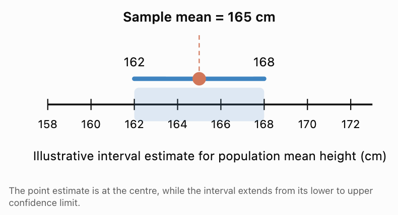
Suppose a random sample of students has an average height of 165 cm.
Point estimate:
μ ≈ 165 cm.
A possible confidence interval might be:
162 cm to 168 cm.
The interval communicates uncertainty about the population mean.
Why Do We Need Confidence Intervals?
Confidence intervals help us:
-
Estimate unknown population parameters.
-
Quantify uncertainty caused by random sampling.
-
Compare the precision of different estimates.
-
Communicate statistical findings.
-
Make decisions using a range rather than a single value.
A point estimate alone may suggest more certainty than the data justify.
A confidence interval provides a more informative summary.
The Structure of a Confidence Interval
Many common confidence intervals follow the form:
Confidence interval = Point estimate ± Margin of error
The margin of error describes how far the interval extends on either side of the point estimate.
More generally:
Margin of error = Critical value × Standard error
Therefore:
Confidence interval = Estimate ± (Critical value × Standard error)
Point Estimate
The sample statistic used to estimate the population parameter.
Critical Value
A multiplier determined by the confidence level and the statistical distribution being used.
Standard Error
A measure of how much a sample statistic varies from sample to sample.
Margin of Error
The amount added to and subtracted from the point estimate to construct the interval.
Worked Example 1: Understanding Margin of Error
A survey estimates that 62% of students prefer digital textbooks.
The reported margin of error is 5 percentage points.
Calculate the interval.
Lower limit:
62% − 5% = 57%.
Upper limit:
62% + 5% = 67%.
Answer: 57% to 67%.
The point estimate is 62%, and the margin of error is 5 percentage points.
This calculation does not by itself establish a confidence level; that depends on how the margin of error was obtained.
Confidence Levels
The confidence level describes the long-run success rate of the method used to construct confidence intervals.
Common confidence levels are:
|
Confidence level |
Approximate z critical value for a two-sided interval |
|---|---|
|
80% |
1.282 |
|
90% |
1.645 |
|
95% |
1.960 |
|
98% |
2.326 |
|
99% |
2.576 |
These z-values apply when a normal critical value is appropriate.
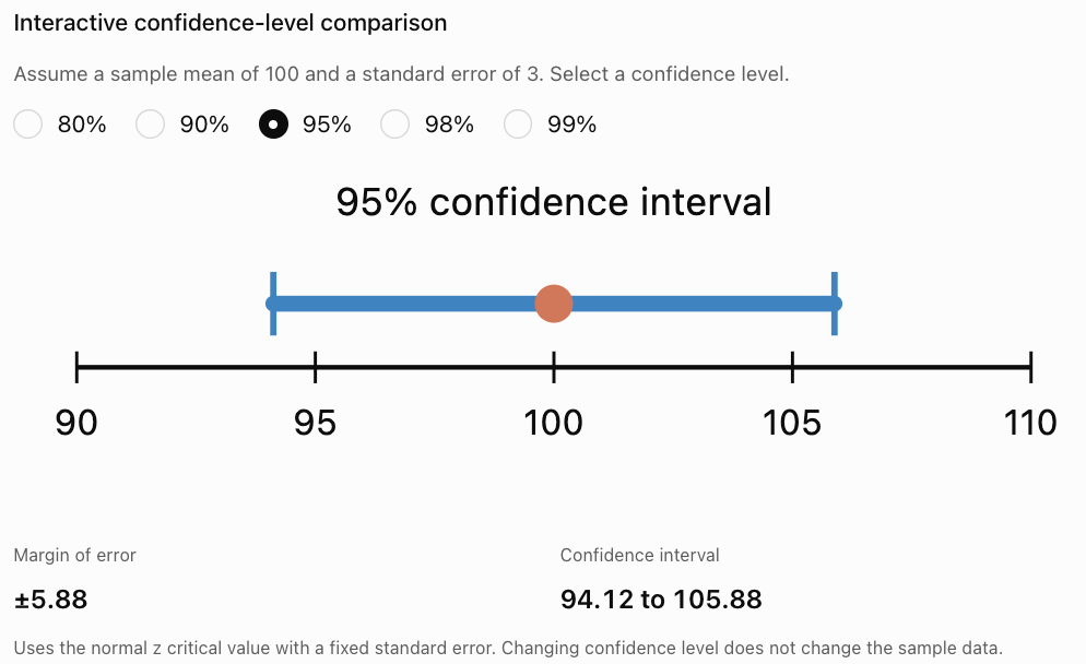
A higher confidence level requires a larger critical value and therefore usually produces a wider interval when the data and method remain unchanged.
What Does 95% Confidence Mean?
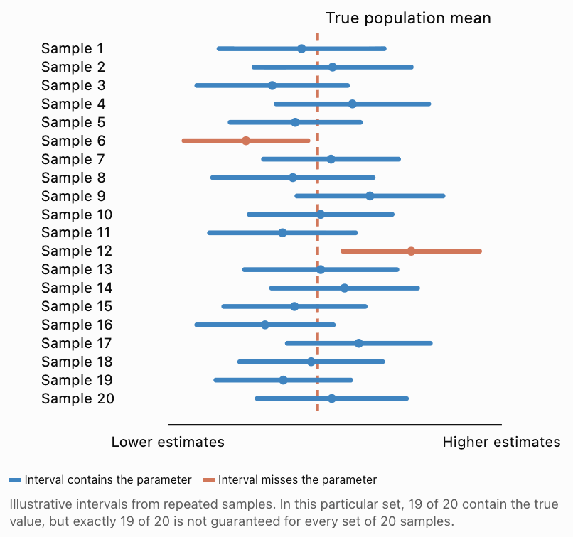
Suppose we repeatedly:
-
Select a random sample from the same population.
-
Calculate a 95% confidence interval using the same valid method.
-
Record whether the interval contains the true population parameter.
Over many repetitions, approximately 95% of the calculated intervals would contain the true parameter.
This is the correct frequentist interpretation of a 95% confidence level.
It does not mean that there is a 95% probability that the fixed population parameter lies inside one particular interval after it has been calculated.
The parameter is treated as fixed; the interval changes from sample to sample.
Repeated 95% confidence intervals (illustrative simulation)
Confidence Level and Interval Width
Explore how the same sample estimate produces different interval widths when the confidence level changes.
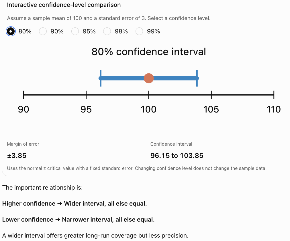
The important relationship is:
Higher confidence → Wider interval, all else equal.
Lower confidence → Narrower interval, all else equal.
A wider interval offers greater long-run coverage but less precision.
Calculating Confidence Intervals for a Population Mean
When estimating a population mean, the appropriate method depends on whether the population standard deviation is known.
Case 1: Population Standard Deviation Is Known
When the population standard deviation σ is known and the sampling distribution of the mean is normal or approximately normal, use the z confidence interval.
Formula:
CI = x̄ ± z* × σ/√n
Where:
-
x̄ = sample mean.
-
z* = critical value.
-
σ = population standard deviation.
-
n = sample size.
-
σ/√n = standard error of the sample mean.
The method assumes independent observations from an appropriate sampling process. A normal population or sufficiently large sample can justify the normal approximation.
Worked Example 2: A 95% Confidence Interval for a Mean
A manufacturer produces batteries.
A random sample of 64 batteries has an average lifetime of 520 hours.
The population standard deviation is known to be 40 hours.
Construct a 95% confidence interval for the population mean battery lifetime.
Step 1: Identify the information
x̄ = 520 hours.
σ = 40 hours.
n = 64.
z* = 1.96.
Step 2: Calculate the standard error
SE = σ/√n
= 40/√64
= 40/8
= 5 hours.
Step 3: Calculate the margin of error
ME = z* × SE
= 1.96 × 5
= 9.8 hours.
Step 4: Calculate the confidence interval
CI = 520 ± 9.8.
Lower limit:
520 − 9.8 = 510.2.
Upper limit:
520 + 9.8 = 529.8.
Answer: 95% CI = (510.2, 529.8) hours.
Interpretation: We are 95% confident that the population mean battery lifetime lies between 510.2 and 529.8 hours, in the sense that the method used has 95% long-run coverage under its assumptions.
Worked Example 3: Comparing 90% and 99% Confidence Intervals
Using the same battery data:
x̄ = 520, SE = 5.
For a 90% interval:
z* = 1.645.
ME = 1.645 × 5 = 8.225.
CI = (511.775, 528.225).
For a 99% interval:
z* = 2.576.
ME = 2.576 × 5 = 12.88.
CI = (507.12, 532.88).
|
Confidence level |
Margin of error |
Confidence interval |
|---|---|---|
|
90% |
8.23 hours |
511.78–528.23 hours |
|
95% |
9.80 hours |
510.20–529.80 hours |
|
99% |
12.88 hours |
507.12–532.88 hours |
Conclusion: The 99% confidence interval is wider because it is designed to achieve a higher long-run coverage rate.
Case 2: Population Standard Deviation Is Unknown
In most real-world investigations, the population standard deviation σ is unknown.
Instead, we use the sample standard deviation s.
For a confidence interval for a population mean, the standard method is the Student's t-distribution.
Formula:
CI = x̄ ± t* × s/√n
Where:
-
x̄ = sample mean.
-
t* = t critical value.
-
s = sample standard deviation.
-
n = sample size.
-
Degrees of freedom = n − 1.
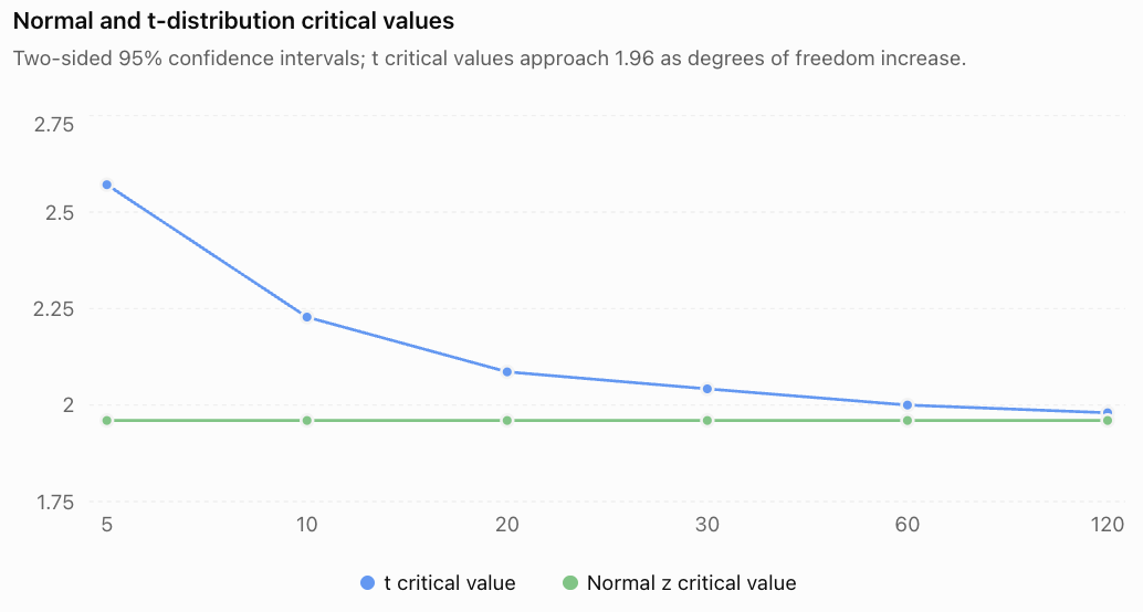
The t-distribution accounts for the additional uncertainty from estimating σ with s.
For small samples, the t-distribution has heavier tails than the standard normal distribution, producing larger critical values.
As the degrees of freedom increase, the t-distribution approaches the normal distribution.
When Is a t-Interval Appropriate?
A one-sample t-interval is appropriate when:
-
The sample is randomly selected or otherwise obtained through a defensible sampling design.
-
Observations are independent or sufficiently close to independent.
-
The population is approximately normal for small samples, with no serious outliers.
-
For larger samples, the sampling distribution of the mean is approximately normal.
For sampling without replacement from a finite population, the sample should generally be a small fraction of the population for the usual independent-observations approximation; a common guideline is no more than 10%.
The t-method does not automatically correct for biased sampling or severe outliers.
Worked Example 4: A 95% t-Confidence Interval
A random sample of 16 students records the following summary statistics for time spent completing a homework task:
Sample mean = 42 minutes.
Sample standard deviation = 8 minutes.
Assume the underlying distribution is approximately normal.
Estimate the population mean completion time using a 95% confidence interval.
Step 1: Identify the information
x̄ = 42.
s = 8.
n = 16.
Degrees of freedom:
df = 16 − 1 = 15.
For 95% confidence and 15 degrees of freedom:
t* ≈ 2.131.
Step 2: Calculate standard error
SE = s/√n
= 8/√16
= 2 minutes.
Step 3: Calculate margin of error
ME = 2.131 × 2
= 4.262 minutes.
Step 4: Construct the interval
CI = 42 ± 4.262.
Lower limit = 37.738.
Upper limit = 46.262.
Answer: 95% CI ≈ (37.74, 46.26) minutes.
Interpretation: We are 95% confident that the population mean homework completion time lies between approximately 37.74 and 46.26 minutes.
The confidence statement concerns the population mean, not the completion time of every individual student.
Worked Example 5: Why We Should Not Automatically Use z = 1.96
Consider the same sample:
x̄ = 42, s = 8, n = 16.
If we incorrectly use z = 1.96:
ME = 1.96 × 8/4
= 3.92.
The resulting interval would be:
(38.08, 45.92).
The correct t-based interval is:
(37.74, 46.26).
The z-based interval is narrower because it fails to account appropriately for the uncertainty in estimating the population standard deviation from this small sample.
Conclusion: When σ is unknown, the t-method is generally the appropriate choice for inference about a population mean.
Confidence Intervals for a Population Proportion
Confidence intervals can also estimate population proportions.
For example:
-
The proportion of students who walk to school.
-
The proportion of voters who support a proposal.
-
The proportion of products that are defective.
-
The proportion of households with internet access.
The sample proportion is:
p̂ = x/n
Where:
-
x = number of successes.
-
n = sample size.
A common introductory method is the normal-approximation, or Wald, interval:
CI = p̂ ± z × √(p̂(1 − p̂)/n)*
This method is easiest to calculate by hand but can perform poorly, particularly for small samples or proportions near 0 or 1. In practice, the Wilson score interval is often preferred.
For introductory Wald calculations, check that:
n p̂ ≥ 10
and
n(1 − p̂) ≥ 10.
These conditions help support the normal approximation, although they do not guarantee ideal coverage.
Worked Example 6: A Confidence Interval for a Proportion
A random sample of 400 students finds that 240 prefer online learning resources.
Construct an approximate 95% confidence interval for the population proportion.
Step 1: Calculate the sample proportion
p̂ = 240/400
= 0.60.
Step 2: Check the approximation
n p̂ = 400 × 0.60 = 240.
n(1 − p̂) = 400 × 0.40 = 160.
Both exceed 10.
Step 3: Calculate standard error
SE = √(0.60 × 0.40/400)
= √0.0006
≈ 0.024495.
Step 4: Calculate margin of error
ME = 1.96 × 0.024495
≈ 0.04801.
Step 5: Calculate interval
CI = 0.60 ± 0.04801.
Lower limit ≈ 0.55199.
Upper limit ≈ 0.64801.
Answer: Approximately (0.552, 0.648), or 55.2% to 64.8%.
Interpretation: We are 95% confident that approximately 55.2% to 64.8% of the population of students prefer online learning resources, assuming the sampling method is appropriate.
Worked Example 7: Estimating a Defect Rate
A manufacturer inspects a random sample of 500 products.
Of these, 25 are defective.
Calculate an approximate 95% confidence interval for the population defect proportion.
Step 1: Sample proportion
p̂ = 25/500 = 0.05.
Step 2: Check approximation
n p̂ = 25.
n(1 − p̂) = 475.
Both are at least 10.
Step 3: Standard error
SE = √(0.05 × 0.95/500)
≈ 0.009747.
Step 4: Margin of error
ME = 1.96 × 0.009747
≈ 0.01910.
Step 5: Interval
CI = 0.05 ± 0.01910.
Answer: Approximately (0.0309, 0.0691), or 3.09% to 6.91%.
The sample defect rate is 5%, but the interval shows that the population defect rate could plausibly differ from that estimate.
Selecting the Appropriate Confidence Interval
|
Situation |
Typical method |
Formula |
|---|---|---|
|
Population mean, σ known |
z interval |
x̄ ± z*σ/√n |
|
Population mean, σ unknown |
t interval |
x̄ ± t*s/√n |
|
Population proportion, introductory approximation |
z/Wald interval |
p̂ ± z*√(p̂(1 − p̂)/n) |
Other methods are needed for differences between groups, paired data, very small proportions, and more complicated sampling designs.
The correct formula depends on the parameter, available information, sampling method, and statistical assumptions.
Estimating Population Parameters
Confidence intervals help us estimate unknown population characteristics without measuring every member of the population.
However, a confidence interval is only as trustworthy as the data and assumptions used to construct it.
Sampling Methods Matter
A random sample is generally preferable to a convenience sample because it reduces the risk of systematic selection bias.
For example, a school wants to estimate the average time students spend using their phones.
Surveying only students who attend a technology club may produce an unrepresentative estimate.
Even a very narrow confidence interval based on biased data may be misleading.
Confidence intervals quantify certain forms of sampling uncertainty; they do not automatically account for bias.
How Sample Size Affects Confidence Intervals
For a mean with known population standard deviation:
ME = z*σ/√n.
The sample size n appears under a square root.
Therefore, increasing the sample size reduces the margin of error, provided other factors remain unchanged.
Worked Example 8: Increasing Sample Size
Suppose:
σ = 20.
Confidence level = 95%.
z* = 1.96.
Compare samples of sizes 25, 100, and 400.
For n = 25:
ME = 1.96 × 20/√25
= 7.84.
For n = 100:
ME = 1.96 × 20/√100
= 3.92.
For n = 400:
ME = 1.96 × 20/√400
= 1.96.
|
Sample size |
Margin of error |
|---|---|
|
25 |
±7.84 |
|
100 |
±3.92 |
|
400 |
±1.96 |
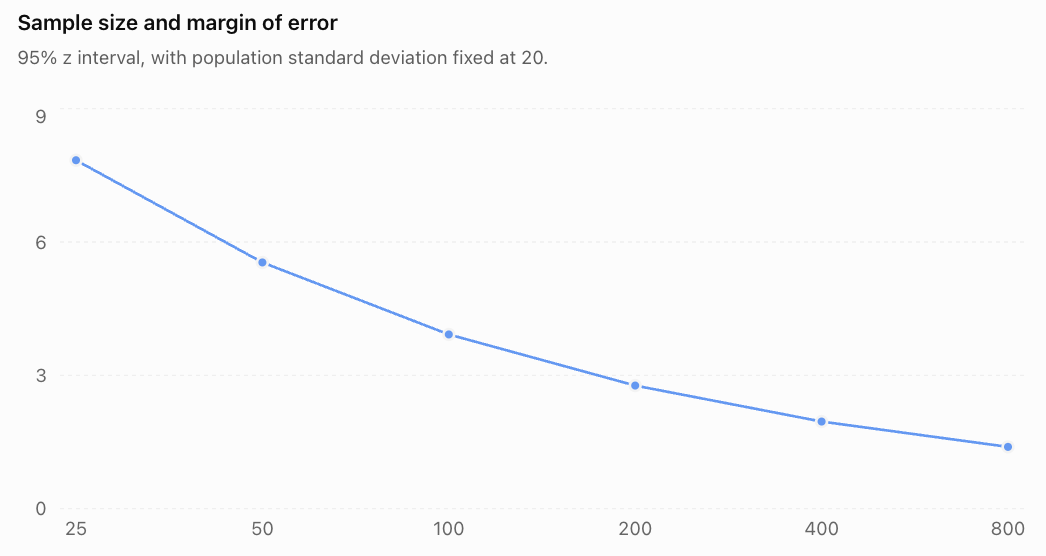
Important result: To halve the margin of error, we generally need four times the sample size.
This is because:
ME ∝ 1/√n.
Calculating a Required Sample Size
Sometimes researchers want to achieve a specified margin of error before collecting data.
For a population mean with known σ:
ME = z*σ/√n.
Rearranging:
√n = z*σ/ME.
Therefore:
**n = (z*σ/ME)²**
Always round the required sample size up to the next whole number.
Worked Example 9: Planning a Survey of a Mean
A researcher wants to estimate the mean mass of a manufactured component.
The population standard deviation is known to be 12 g.
The researcher wants a 95% confidence interval with margin of error no greater than 3 g.
Find the required sample size.
Step 1: Identify the values
z* = 1.96.
σ = 12.
ME = 3.
Step 2: Substitute
n = (1.96 × 12/3)²
= 7.84²
= 61.4656.
Step 3: Round up
Answer: At least 62 components.
Rounding down would not guarantee the target margin of error.
Sample Size for a Population Proportion
For the introductory normal-approximation method, a planning formula is:
**n = z*²p₀(1 − p₀)/ME²**
Where p₀ is an anticipated population proportion.
If no reasonable estimate of the proportion is available, use:
p₀ = 0.5.
This produces the largest value of p₀(1 − p₀) and therefore a conservative sample size under this formula.
Worked Example 10: Planning an Opinion Survey
A researcher wants to estimate a population proportion with:
-
95% confidence.
-
Margin of error no greater than 4 percentage points.
-
No prior estimate of the proportion.
Use p₀ = 0.5.
n = 1.96² × 0.5 × 0.5 / 0.04²
= 3.8416 × 0.25 / 0.0016
= 600.25.
Round up:
Answer: At least 601 respondents.
This assumes a simple random sampling framework and does not include adjustments for nonresponse, clustering, or other design effects.
Interpreting Confidence Intervals Correctly
Calculating a confidence interval is only one part of the statistical process.
A complete interpretation must identify:
-
The population being studied.
-
The parameter being estimated.
-
The confidence level.
-
The lower and upper limits.
-
The appropriate uncertainty statement.
Example of Good Communication
Suppose a 95% confidence interval for the mean daily screen time of students at a school is:
(2.4, 3.1) hours.
A suitable statement is:
"Based on the sample, we are 95% confident that the mean daily screen time of all students at the school is between 2.4 and 3.1 hours."
This identifies the population, parameter, confidence level, and interval.
Statements to Avoid
Incorrect: "95% of students have screen times between 2.4 and 3.1 hours."
The interval concerns the population mean, not the distribution of individual observations.
Incorrect: "There is a 95% probability that the true mean is between 2.4 and 3.1 hours."
Under the usual frequentist interpretation, the parameter is fixed and the confidence procedure has a long-run coverage rate of 95%.
Incorrect: "The population mean must be exactly 2.75 hours."
The midpoint is the point estimate, not necessarily the true population mean.
Confidence Intervals and Practical Decisions
Suppose a manufacturer requires the mean strength of a material to exceed 50 MPa.
A 95% confidence interval for the population mean is:
(52, 58) MPa.
The entire interval is above 50 MPa.
This provides statistical evidence that the population mean exceeds the required threshold, under the model assumptions.
Now consider another interval:
(47, 57) MPa.
This interval includes values below and above 50 MPa.
The result is less conclusive about whether the population mean exceeds the requirement.
However, confidence intervals for the mean do not establish that every individual product meets a strength requirement.
Worked Example 11: Comparing Two Estimates
Two schools estimate average student travel times.
School A:
95% CI = (24, 30) minutes.
School B:
95% CI = (29, 37) minutes.
School A's interval is narrower.
School B's estimated mean is higher.
The intervals overlap between 29 and 30 minutes.
Can we conclude that the population means are equal?
No.
Overlapping confidence intervals do not prove that two population means are equal.
Nor does overlap alone determine whether their difference is statistically significant.
A formal comparison should use a confidence interval or test for the difference between population means, taking the sampling design into account.
The Accuracy and Limitations of Confidence Intervals
Sampling Error
Sampling error occurs because a sample statistic differs from the population parameter due to random variation.
A confidence interval helps quantify this uncertainty.
Sampling Bias
Sampling bias occurs when the sampling method systematically overrepresents or underrepresents part of the population.
Increasing sample size does not necessarily remove sampling bias.
Nonresponse Bias
If selected participants do not respond and their characteristics differ systematically from those who do, the estimate may be biased.
Measurement Error
Inaccurate measuring instruments or unclear survey questions may distort results.
Distributional Assumptions
Some confidence interval formulas rely on assumptions about normality, independence, or sufficiently large samples.
Confidence Versus Precision
A narrow interval is more precise than a wide interval, but precision does not automatically imply accuracy.
A very precise estimate from biased data may still be wrong.
Worked Example 12: A Misleading Survey
A school surveys 1000 students who voluntarily respond to a website poll about homework.
The sample indicates that 80% of respondents dislike homework.
The survey produces a very small nominal margin of error under a simple random-sample formula.
Can the school confidently conclude that approximately 80% of all students dislike homework?
Not necessarily.
Students with strong opinions may be more likely to participate.
This creates possible voluntary-response bias.
The large sample size reduces random sampling variability under a random-sampling model, but it does not correct the nonrandom selection mechanism.
Conclusion: The survey may produce a precise-looking estimate that does not accurately represent the population.
Real-World Applications
Scientific research
Researchers use confidence intervals to report estimates of experimental measurements and population characteristics.
Manufacturing
Engineers estimate average product dimensions, strengths, and defect rates.
Education
Schools estimate average achievement, study habits, and student preferences.
Public health
Researchers report uncertainty in estimated health outcomes, proportions, and treatment effects.
Integrated Investigation: Student Study Time
A school wants to estimate the mean daily study time of its students.
A random sample of 100 students provides:
x̄ = 92 minutes.
s = 25 minutes.
Assume the observations are independent and the t-method is appropriate.
Part A: Identify the Parameter
The population parameter is:
μ = mean daily study time of all students at the school.
The sample mean of 92 minutes is the point estimate.
Part B: Calculate Standard Error
SE = s/√n
= 25/√100
= 2.5 minutes.
Part C: Find the Critical Value
For 95% confidence:
df = 100 − 1 = 99.
t* ≈ 1.984.
Part D: Calculate Margin of Error
ME = 1.984 × 2.5
= 4.96 minutes.
Part E: Construct the Interval
CI = 92 ± 4.96.
Answer: (87.04, 96.96) minutes.
Part F: Interpret
We are 95% confident that the mean daily study time of all students at the school lies between approximately 87.0 and 97.0 minutes.
Part G: Evaluate the Estimate
The result assumes the sample is representative and the measurements are reliable.
Potential limitations include:
-
Students may misreport study time.
-
Daily study time may vary by weekday.
-
The sample may exclude absent students.
-
The sample may not represent all grade levels equally.
A more detailed study could use stratified random sampling across grade levels and collect measurements over several days.
This investigation demonstrates the complete statistical process: identifying a parameter, calculating an interval, interpreting the result, and evaluating its reliability.
Common Mistakes
Mistake 1: Treating a Confidence Interval as an Interval for Individual Values
A confidence interval for μ estimates the population mean, not where most individual observations lie.
Mistake 2: Saying the Population Parameter Has a 95% Probability of Being Inside a Calculated 95% Interval
In frequentist statistics, 95% describes the long-run coverage of the procedure.
Mistake 3: Confusing the Sample Mean with the Population Mean
x̄ is an estimate of μ, not necessarily its exact value.
Mistake 4: Using the Wrong Standard Error
For a sample mean with known σ:
SE = σ/√n.
For a sample proportion under the introductory approximation:
SE = √(p̂(1 − p̂)/n).
Mistake 5: Forgetting the Square Root of Sample Size
The standard error of a mean is not σ/n.
Mistake 6: Using z When a t-Interval Is Appropriate
For a population mean with unknown σ, the t-distribution is generally used.
Mistake 7: Forgetting Degrees of Freedom
For a one-sample t-interval:
df = n − 1.
Mistake 8: Confusing Confidence Level and Margin of Error
Confidence level describes long-run coverage.
Margin of error describes interval half-width.
Mistake 9: Assuming Higher Confidence Produces a Narrower Interval
Higher confidence generally requires a wider interval for fixed data.
Mistake 10: Assuming a Large Sample Eliminates Bias
A large biased sample may still produce a misleading estimate.
Mistake 11: Using a Normal Approximation for an Unsuitable Proportion Sample
Small samples and proportions near 0 or 1 can make the basic Wald interval unreliable.
Mistake 12: Rounding Too Early
Keep sufficient precision until the final result.
Mistake 13: Reporting Proportions Incorrectly
An interval of (0.42, 0.56) corresponds to 42%–56%, not 0.42%–0.56%.
Mistake 14: Forgetting to Identify the Population
A confidence interval should specify whose mean or proportion is being estimated.
Mistake 15: Interpreting Overlapping Intervals as Proof of Equality
Overlapping confidence intervals do not prove equal population parameters.
Mistake 16: Treating a Confidence Interval as a Guarantee
Even a valid 99% confidence procedure can produce an interval that misses the true parameter.
Mistake 17: Ignoring Independence
Dependent observations can invalidate standard error formulas that assume independence.
Mistake 18: Confusing Statistical and Practical Importance
An estimated difference can be statistically distinguishable from zero but too small to matter in practice.
Mistake 19: Rounding Required Sample Size Down
Always round up when calculating a minimum required sample size.
Mistake 20: Failing to Explain Assumptions
A complete statistical conclusion should acknowledge relevant sampling and modelling limitations.
Key Terms
-
Population: The complete group being studied.
-
Sample: A subset of the population.
-
Parameter: A numerical characteristic of a population.
-
Statistic: A numerical characteristic calculated from sample data.
-
Population Mean (μ): The mean of the entire population.
-
Sample Mean (x̄): The mean calculated from a sample.
-
Population Proportion (p): The proportion of the population with a particular characteristic.
-
Sample Proportion (p̂): The proportion of sampled observations with that characteristic.
-
Population Standard Deviation (σ): A measure of variability in the population.
-
Sample Standard Deviation (s): A measure of variability in a sample.
-
Point Estimate: A single-value estimate of a population parameter.
-
Interval Estimate: A range used to estimate a population parameter.
-
Confidence Interval: An interval constructed by a procedure with a specified long-run coverage probability.
-
Confidence Level: The intended long-run proportion of intervals that contain the parameter.
-
Critical Value: A distribution-based multiplier used in constructing an interval.
-
Standard Error: The standard deviation of a statistic's sampling distribution, or an estimate of it.
-
Margin of Error: The distance from the point estimate to an interval endpoint for a symmetric interval.
-
Lower Confidence Limit: The lower endpoint of a confidence interval.
-
Upper Confidence Limit: The upper endpoint of a confidence interval.
-
Sampling Variability: Differences in statistics obtained from different samples.
-
Sampling Distribution: The probability distribution of a statistic across repeated samples.
-
Normal Distribution: A symmetric, bell-shaped probability distribution.
-
z-Score: A standardized value relative to a normal distribution.
-
Student's t-Distribution: A family of distributions used in inference about means when σ is estimated.
-
Degrees of Freedom: A quantity determining the appropriate t-distribution.
-
Random Sampling: Sampling using a chance-based selection mechanism.
-
Sampling Bias: Systematic distortion caused by the selection process.
-
Nonresponse Bias: Bias caused by differences between respondents and nonrespondents.
-
Measurement Error: Inaccuracy in recorded observations.
-
Normal Approximation: Using a normal distribution to approximate a sampling distribution.
-
Wald Interval: A basic normal-approximation confidence interval for a proportion.
-
Wilson Score Interval: An alternative confidence interval for a proportion with generally better coverage properties.
-
Statistical Inference: Using sample data to draw conclusions about populations.
-
Precision: The degree of uncertainty or variability in an estimate.
-
Coverage Probability: The probability that an interval-construction procedure includes the true parameter across repeated samples.
-
Statistical Assumption: A condition required for a statistical method to work as intended.
Key Takeaways
-
Confidence intervals estimate unknown population parameters.
-
A sample statistic provides a point estimate.
-
An interval estimate communicates sampling uncertainty.
-
Many confidence intervals have the form estimate ± margin of error.
-
Margin of error depends on a critical value and standard error.
-
A 95% confidence procedure has approximately 95% long-run coverage under its assumptions.
-
A confidence interval for a mean does not describe the spread of individual observations.
-
Higher confidence levels generally produce wider intervals.
-
Larger sample sizes generally produce narrower intervals.
-
Standard errors for sample means decrease approximately with 1/√n.
-
A z-interval can be used for a mean when σ is known and its assumptions hold.
-
A t-interval is generally used for a mean when σ is unknown.
-
The sample proportion estimates the population proportion.
-
The basic proportion z-interval requires care, especially for small samples.
-
Sample size can be planned using a target margin of error.
-
Random sampling helps support valid population inference.
-
Confidence intervals do not automatically correct sampling bias.
-
Statistical precision does not guarantee accuracy.
-
Interval interpretations should identify the population, parameter, and confidence level.
-
Good statistical communication includes assumptions, uncertainty, and limitations.
Check Your Understanding
Show all calculations. Select an appropriate method, state the population parameter, and interpret each interval in context.
Question 1: Purpose of Confidence Intervals
Explain why a confidence interval is often more informative than a point estimate.
Question 2: Margin of Error
A survey estimates that 58% of students use public transport.
The reported margin of error is 4 percentage points.
Calculate the interval endpoints.
Question 3: Confidence Levels
Explain the meaning of a 95% confidence level.
Why does a 99% confidence interval generally have a greater width than a 95% confidence interval based on the same data?
Question 4: z-Interval for a Mean
A random sample of 100 products has mean mass 250 g.
The population standard deviation is known to be 20 g.
Calculate a 95% confidence interval for the population mean mass.
Question 5: 90% Confidence Interval
A random sample of 64 measurements has mean 120 and known population standard deviation 16.
Calculate a 90% confidence interval.
Use z* = 1.645.
Question 6: t-Interval for a Mean
A random sample of 25 students has mean test score 72 and sample standard deviation 10.
Assume the t-method is appropriate.
Calculate a 95% confidence interval.
Use t* = 2.064.
Question 7: Degrees of Freedom
A random sample contains 18 observations.
What degrees of freedom should be used for a one-sample t confidence interval?
Question 8: Proportion Confidence Interval
In a random sample of 500 students, 300 prefer digital assignments.
Calculate an approximate 95% confidence interval for the population proportion using the introductory normal approximation.
Question 9: Product Defect Rate
A random sample of 400 products contains 32 defective products.
Calculate an approximate 95% confidence interval for the population defect proportion.
Question 10: Sample Size and Precision
A researcher uses a 95% z-interval for a mean with σ = 15.
Calculate the margin of error for:
a) n = 25.
b) n = 100.
Explain the relationship.
Question 11: Planning Sample Size
A researcher wants to estimate a population mean with:
σ = 18.
Confidence level = 95%.
Desired margin of error = 4.
Calculate the minimum sample size.
Question 12: Survey Sample Size
A researcher wants to estimate a population proportion at 95% confidence with a margin of error no greater than 5 percentage points.
No previous estimate of the proportion is available.
Calculate the minimum sample size using p₀ = 0.5.
Question 13: Interpreting an Interval
A 95% confidence interval for mean weekly exercise time is:
(3.2, 4.6) hours.
Explain what this interval means and identify one incorrect interpretation.
Question 14: Evaluating Bias
A school surveys only members of its sports teams to estimate the average weekly exercise time of all students.
Explain why the resulting confidence interval may be misleading.
Question 15: Comprehensive Investigation
A school selects a random sample of 36 students to estimate mean daily reading time.
The sample has:
x̄ = 48 minutes.
s = 12 minutes.
Assume the t-method is appropriate.
For 95% confidence and 35 degrees of freedom, use:
t* = 2.030.
Calculate:
a) The standard error.
b) The margin of error.
c) The confidence interval.
d) A complete interpretation.
e) Two limitations of the investigation.
Fully Worked Answers
Answer 1: Purpose of Confidence Intervals
A point estimate provides one numerical estimate of a population parameter.
A confidence interval provides a range of plausible parameter values and communicates uncertainty caused by sampling variability.
For example, a sample mean of 80 minutes does not reveal how precisely the population mean has been estimated.
A confidence interval of 76–84 minutes communicates more information about the estimate's uncertainty.
Answer 2: Margin of Error
Point estimate = 58%.
Margin of error = 4 percentage points.
Lower limit:
58% − 4% = 54%.
Upper limit:
58% + 4% = 62%.
Answer: 54% to 62%.
The confidence level cannot be determined from these values alone.
Answer 3: Confidence Levels
A 95% confidence level means that if we repeatedly selected samples and calculated intervals using the same valid procedure, approximately 95% of those intervals would contain the true population parameter.
A 99% interval uses a larger critical value than a 95% interval.
Since:
ME = Critical value × Standard error,
the 99% interval is generally wider for the same data.
This increases long-run coverage but reduces precision.
Answer 4: z-Interval for a Mean
Given:
x̄ = 250 g.
σ = 20 g.
n = 100.
z* = 1.96.
Step 1: Standard error
SE = 20/√100
= 2 g.
Step 2: Margin of error
ME = 1.96 × 2
= 3.92 g.
Step 3: Confidence interval
CI = 250 ± 3.92.
Lower limit = 246.08 g.
Upper limit = 253.92 g.
Answer: 95% CI = (246.08, 253.92) g.
We are 95% confident that the population mean product mass is between 246.08 g and 253.92 g, using the standard long-run interpretation.
Answer 5: 90% Confidence Interval
Given:
x̄ = 120.
σ = 16.
n = 64.
z* = 1.645.
Step 1: Standard error
SE = 16/√64
= 16/8
= 2.
Step 2: Margin of error
ME = 1.645 × 2
= 3.29.
Step 3: Interval
CI = 120 ± 3.29.
Answer: 90% CI = (116.71, 123.29).
Answer 6: t-Interval for a Mean
Given:
x̄ = 72.
s = 10.
n = 25.
t* = 2.064.
Step 1: Standard error
SE = 10/√25
= 2.
Step 2: Margin of error
ME = 2.064 × 2
= 4.128.
Step 3: Confidence interval
CI = 72 ± 4.128.
Lower limit = 67.872.
Upper limit = 76.128.
Answer: 95% CI ≈ (67.87, 76.13).
We are 95% confident that the population mean test score is between approximately 67.87 and 76.13 points, assuming the sampling and t-interval conditions are satisfied.
Answer 7: Degrees of Freedom
For a one-sample t-interval:
df = n − 1.
n = 18.
df = 18 − 1.
Answer: 17 degrees of freedom.
Answer 8: Proportion Confidence Interval
Given:
x = 300.
n = 500.
Step 1: Sample proportion
p̂ = 300/500
= 0.60.
Step 2: Standard error
SE = √(0.60 × 0.40/500)
= √0.00048
≈ 0.021909.
Step 3: Margin of error
ME = 1.96 × 0.021909
≈ 0.04294.
Step 4: Confidence interval
CI = 0.60 ± 0.04294.
Lower limit ≈ 0.55706.
Upper limit ≈ 0.64294.
Answer: Approximately (0.5571, 0.6429), or 55.71% to 64.29%.
We are 95% confident that the population proportion preferring digital assignments is approximately 55.71% to 64.29%, assuming the method is appropriate.
Answer 9: Product Defect Rate
Given:
x = 32 defective products.
n = 400.
Step 1: Sample proportion
p̂ = 32/400
= 0.08.
Step 2: Standard error
SE = √(0.08 × 0.92/400)
= √0.000184
≈ 0.013565.
Step 3: Margin of error
ME = 1.96 × 0.013565
≈ 0.02659.
Step 4: Interval
CI = 0.08 ± 0.02659.
Lower limit ≈ 0.05341.
Upper limit ≈ 0.10659.
Answer: Approximately 5.34% to 10.66%.
The population defect rate is estimated to lie within this interval using the introductory 95% normal-approximation method.
Answer 10: Sample Size and Precision
Given:
σ = 15.
z* = 1.96.
a) n = 25
ME = 1.96 × 15/√25
= 1.96 × 3
Answer: 5.88.
b) n = 100
ME = 1.96 × 15/√100
= 1.96 × 1.5
Answer: 2.94.
Explanation
The sample size increased from 25 to 100, a factor of 4.
The margin of error decreased from 5.88 to 2.94, a factor of 2.
This agrees with:
ME ∝ 1/√n.
Answer 11: Planning Sample Size
Given:
σ = 18.
z* = 1.96.
Desired ME = 4.
Use:
n = (z*σ/ME)².
Substitute:
n = (1.96 × 18/4)²
= 8.82²
= 77.7924.
Round up.
Answer: At least 78 observations.
Answer 12: Survey Sample Size
Given:
z* = 1.96.
ME = 0.05.
p₀ = 0.5.
Use:
n = z*²p₀(1 − p₀)/ME².
Substitute:
n = 1.96² × 0.5 × 0.5 / 0.05²
= 3.8416 × 0.25 / 0.0025
= 384.16.
Round up.
Answer: At least 385 respondents.
This is the introductory sample-size calculation for a simple random sample and does not account for nonresponse or complex survey design.
Answer 13: Interpreting an Interval
The 95% confidence interval is:
(3.2, 4.6) hours.
Correct interpretation:
We are 95% confident that the population mean weekly exercise time is between 3.2 and 4.6 hours, meaning the interval was calculated using a procedure with 95% long-run coverage under its assumptions.
Incorrect interpretation:
"95% of individuals exercise between 3.2 and 4.6 hours per week."
The confidence interval estimates the population mean, not the distribution of individual exercise times.
Answer 14: Evaluating Bias
The sample includes only members of school sports teams.
These students may exercise more frequently than students who do not participate in sports teams.
Therefore, the sample may systematically overestimate the average exercise time of the entire school population.
Even if the confidence interval is narrow, it may not accurately represent all students.
Conclusion: The investigation suffers from potential selection bias.
A better method would be to select a random sample from the entire student population, possibly stratifying by grade level.
Answer 15: Comprehensive Investigation
Given:
x̄ = 48 minutes.
s = 12 minutes.
n = 36.
t* = 2.030.
a) Standard error
SE = s/√n
= 12/√36
= 12/6
Answer: 2 minutes.
b) Margin of error
ME = t* × SE
= 2.030 × 2
Answer: 4.06 minutes.
c) Confidence interval
CI = 48 ± 4.06.
Lower limit:
48 − 4.06 = 43.94.
Upper limit:
48 + 4.06 = 52.06.
Answer: 95% CI = (43.94, 52.06) minutes.
d) Interpretation
Based on the sample, we are 95% confident that the mean daily reading time of all students at the school is between 43.94 and 52.06 minutes.
This means the interval was constructed using a procedure that would contain the true population mean in approximately 95% of repeated samples, assuming its conditions hold.
e) Two limitations
1. Self-reporting or measurement error: If students estimate their own reading time, the reported values may be inaccurate.
2. Representativeness: Even a random sample may be affected by nonresponse or incomplete coverage of the student population.
A more reliable investigation could use a clearly defined sampling frame, consistent measurement procedures, and repeated observations over several days.
Final Course Connections
Confidence intervals connect probability, sampling distributions, descriptive statistics, and statistical inference.
They allow us to move beyond reporting a single sample result and instead communicate a range of plausible values for an unknown population parameter.
The most important skills are selecting an appropriate method, calculating the standard error and margin of error, interpreting the confidence level correctly, and evaluating the assumptions behind the estimate.
A confidence interval is not a guarantee of the true value. It is a statistically justified way to communicate uncertainty.
This completes Confidence Intervals, covering all five learning targets with detailed explanations, 12 worked examples, diagrams and charts, real-world applications, common mistakes, key terms, key takeaways, and 15 practice questions with fully worked answers.