4. Shape of Distributions

Shape of Distributions

Introduction

When analysing data, it is important to understand not only the individual values but also how those values are distributed.

The shape of a distribution describes how frequently different values occur and how those values are arranged across a dataset.

Two datasets may have the same mean or median but very different distributions. One might be symmetrical, another might be strongly skewed, and another might contain unusual observations called outliers.

Understanding distribution shape helps us:

• Recognise patterns in data.

• Identify symmetric and skewed distributions.

• Detect unusual observations.

• Interpret measures such as the mean, median, and standard deviation.

• Compare datasets more accurately.

• Decide which statistical measures best describe the data.

Distribution shapes are used in education, economics, medicine, environmental science, manufacturing, and many other fields.

What Is a Distribution?

A distribution describes how the values of a variable are spread across a dataset.

Consider the following examination scores:

45, 52, 58, 63, 67, 70, 72, 75, 79, 84, 91

We can analyse these scores by asking:

• Where are most of the scores concentrated?

• Are the scores spread evenly?

• Are there more high scores or low scores?

• Are any scores unusually far from the others?

• Does the distribution have one peak or several peaks?

The answers help us understand the shape of the distribution.

Frequency Distributions

A frequency distribution records how often values or groups of values occur.

For example:

This table shows that the greatest concentration of scores is between 70 and 79.

A histogram can make the pattern easier to recognise.

Using Histograms to Examine Shape

A histogram displays the frequencies of numerical data grouped into intervals.

The horizontal axis represents numerical intervals.

The vertical axis represents frequency.

Unlike a typical bar chart for categories, histogram bars normally touch because the intervals represent a continuous numerical scale.

Example

Consider the following grouped data:

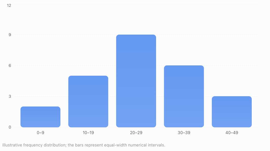
Most observations occur near the middle of the range.

There are fewer observations at the lower and upper ends.

Important Features to Examine

When studying a histogram, look for:

• Centre: Where the typical values are located.

• Spread: How widely the observations vary.

• Shape: Whether the distribution is symmetric or skewed.

• Peaks: Where observations are most concentrated.

• Gaps: Intervals containing few or no observations.

• Outliers: Observations unusually distant from the rest.

These features provide a more complete description than the mean alone.

Symmetric Distributions

A symmetric distribution has approximately the same shape on both sides of its centre.

If the distribution were folded vertically through its centre, the two sides would approximately match.

Symmetric distributions have balanced left and right tails.

Example

Consider:

2, 4, 6, 8, 10, 12, 14

The values are evenly arranged around 8.

The mean is:

(2 + 4 + 6 + 8 + 10 + 12 + 14)/7 = 8

The median is also 8.

This dataset is symmetric around 8.

A Symmetric Frequency Distribution

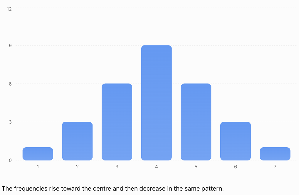
The frequencies rise toward the centre and then decrease in the same pattern.

Characteristics of Symmetric Distributions

• The left and right sides have similar shapes.

• The tails are approximately balanced.

• The mean and median are often close together.

• A symmetric distribution may have one peak, multiple peaks, or a flat shape.

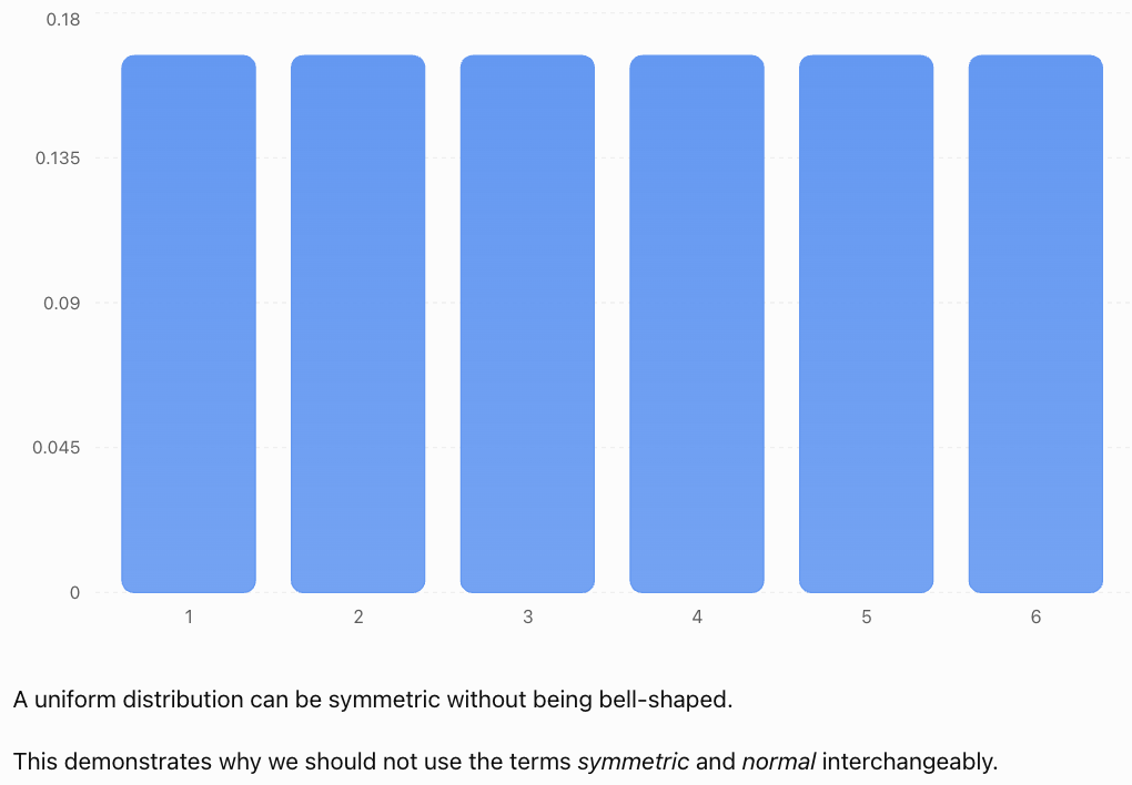
Important: Symmetry does not automatically mean the distribution is normal or bell-shaped.

The Normal Distribution

One important symmetric distribution is the normal distribution.

It is often called the bell-shaped distribution because of its characteristic appearance.

Characteristics

A normal distribution:

• Is symmetric around its mean.

• Has one central peak.

• Has mean, median, and mode at the same location.

• Has tails that extend in both directions.

• Has a shape determined by its mean and standard deviation.

Many measurements are approximately normal under suitable conditions, although real datasets are rarely perfectly normal.

Examples may include some measurement errors and certain biological characteristics within appropriately defined populations.

The Empirical Rule

For a normal distribution:

• Approximately 68% of observations lie within one standard deviation of the mean.

• Approximately 95% lie within two standard deviations.

• Approximately 99.7% lie within three standard deviations.

This is known as the 68–95–99.7 rule.

It applies to normal distributions, not automatically to every symmetric distribution.

Uniform Distributions

A uniform distribution has approximately equal frequencies across its possible values or intervals.

For example, a fair six-sided die has an equal probability of producing each number from 1 to 6.

The theoretical probabilities are:

Outcome	Probability
1	1/6
2	1/6
3	1/6
4	1/6
5	1/6
6	1/6

Skewed Distributions

A skewed distribution is asymmetric.

One side extends farther than the other, producing a longer tail.

There are two main types:

• Right-skewed distributions.

• Left-skewed distributions.

The direction of skewness is named after the direction of the longer tail, not the location of the tallest bars.

Right-Skewed Distributions

A right-skewed distribution, also called a positively skewed distribution, has a longer tail extending toward larger values.

Most observations are concentrated toward the lower end.

A smaller number of large observations extend the distribution to the right.

Example: Household Incomes

In many populations, most households earn low-to-middle incomes relative to a smaller number of very high-income households.

Example Dataset

20, 22, 23, 24, 25, 26, 28, 32, 80

Most values are between 20 and 32.

The value 80 is much larger than the others.

Calculate the Mean

Sum = 280

Mean = 280/9

Mean ≈ 31.11

Find the Median

There are nine observations.

The fifth value is 25.

Median = 25

The mean is larger than the median because the unusually high value pulls the mean upward.

Characteristics

• Most values are concentrated toward the left.

• The tail extends toward the right.

• Large values may increase the mean.

• The mean is often greater than the median.

Important Qualification

Mean > median is a common pattern in right-skewed distributions, but it is not a guaranteed rule for every possible dataset.

Distribution shape should be judged primarily from the data or graph, not only by comparing two summary statistics.

Left-Skewed Distributions

A left-skewed distribution, also called a negatively skewed distribution, has a longer tail extending toward smaller values.

Most observations are concentrated toward the higher end.

A smaller number of low observations extend the distribution to the left.

Example: An Easy Examination

Suppose most students score highly on an examination, but a few students receive much lower marks.

The distribution may be left-skewed.

Example Dataset

20, 68, 72, 74, 76, 78, 79, 80, 82

Calculate the Mean

Sum = 629

Mean = 629/9

Mean ≈ 69.89

Find the Median

The fifth value is 76.

Median = 76

The mean is smaller than the median because the low value pulls the mean downward.

Characteristics

• Most observations are concentrated toward the right.

• The tail extends toward the left.

• Low values may decrease the mean.

• The mean is often less than the median.

Comparing Symmetric and Skewed Distributions

Remember

The direction of skewness is determined by the longer tail.

Understanding Outliers

An outlier is an observation that lies unusually far from the main group of data.

Outliers may be much higher or much lower than most observations.

Example

Consider:

12, 13, 14, 15, 15, 16, 17, 18, 65

Most values are between 12 and 18.

The value 65 is unusually large.

It is a possible outlier.

Possible Causes of Outliers

Outliers may result from:

• Measurement errors.

• Data entry mistakes.

• Unusual but genuine observations.

• Equipment problems.

• Rare events.

• Natural variation.

• Observations from a different population.

Important Observation

An outlier is not necessarily an error.

A very high examination score, an unusually tall person, or an extreme weather event may be genuine.

Outliers should be investigated before deciding whether to exclude them.

Identifying Outliers Using the IQR Method

One common method uses the interquartile range.

The interquartile range measures the spread of the middle 50% of the data.

IQR = Q₃ − Q₁

Potential outliers are identified using two boundaries called fences.

Lower Fence

Lower fence = Q₁ − 1.5 × IQR

Upper Fence

Upper fence = Q₃ + 1.5 × IQR

Values below the lower fence or above the upper fence are flagged as potential outliers.

Worked Example

Consider:

4, 5, 6, 7, 8, 9, 10, 11, 12, 30

Step 1: Find the Median

Median = (8 + 9)/2

Median = 8.5

Step 2: Find the Quartiles

Using the median-of-halves convention:

Lower half:

4, 5, 6, 7, 8

Q₁ = 6

Upper half:

9, 10, 11, 12, 30

Q₃ = 11

Step 3: Calculate the IQR

IQR = 11 − 6

IQR = 5

Step 4: Calculate the Fences

Lower fence = 6 − 1.5(5)

Lower fence = −1.5

Upper fence = 11 + 1.5(5)

Upper fence = 18.5

Step 5: Identify Outliers

Any value below −1.5 or above 18.5 is flagged.

The value 30 is above 18.5.

Therefore, 30 is a potential outlier.

Important Note

There are several accepted methods for calculating quartiles. The median-of-halves convention is used in this example. Different quartile conventions may produce slightly different fences, particularly for small datasets.

Identifying Unusual Values Using z-Scores

Another method uses standardized scores.

The z-score formula is:

z = (x − μ)/σ

A z-score describes how many standard deviations an observation lies above or below the mean.

Common Screening Guidelines

• |z| > 2 may indicate an unusually distant observation.

• |z| > 3 is sometimes used to flag more extreme observations.

These are guidelines, not universal definitions of outliers.

Worked Example

A dataset has:

Mean = 50

Standard deviation = 10

An observation has value 85.

Calculate:

z = (85 − 50)/10

z = 35/10

z = 3.5

The observation is 3.5 standard deviations above the mean.

It may be considered unusually high.

Limitations

The mean and standard deviation can themselves be affected by extreme observations.

For strongly skewed datasets, IQR-based methods may be more appropriate than simple z-score thresholds.

How Outliers Affect the Mean and Median

Outliers can strongly affect some measures of centre.

Consider:

10, 12, 14, 16, 18

Original Mean

Mean = (10 + 12 + 14 + 16 + 18)/5

Mean = 70/5

Mean = 14

Original Median

Median = 14

Now replace the final value, 18, with 100.

New dataset:

10, 12, 14, 16, 100

New Mean

Mean = 152/5

Mean = 30.4

New Median

Median = 14

Interpretation

The mean increases substantially from 14 to 30.4.

The median remains unchanged.

This shows that:

• The mean is sensitive to extreme values.

• The median is more resistant to extreme values.

For skewed distributions or datasets containing outliers, the median may better represent a typical observation.

Choosing Between Mean and Median

The most appropriate measure of centre depends on the distribution.

Symmetric Distributions

For approximately symmetric distributions without extreme outliers, the mean is often a useful measure of centre.

Skewed Distributions

For strongly skewed distributions, the median is often more representative.

Distributions with Outliers

The median is usually less affected by extreme observations.

Example: Household Income

Suppose five households earn:

$35,000, $40,000, $45,000, $50,000, $500,000

The mean is:

(35,000 + 40,000 + 45,000 + 50,000 + 500,000)/5

Mean = $134,000

The median is:

$45,000

The median gives a better indication of the income of a typical household in this small group.

The mean is much higher because of one unusually large income.

Unimodal, Bimodal, and Multimodal Distributions

The number of peaks is another important feature of distribution shape.

A mode is a value or category with the highest frequency.

Unimodal Distribution

A unimodal distribution has one main peak.

Many approximately normal distributions are unimodal.

Bimodal Distribution

A bimodal distribution has two distinct peaks.

This may occur when data come from two different groups.

Multimodal Distribution

A multimodal distribution has more than two peaks.

Example: Two Student Groups

Suppose one group of students scores mainly between 40 and 50, while another group scores mainly between 80 and 90.

Combining the results may produce two peaks.

This could indicate two distinct groups within the dataset.

Important Observation

A bimodal distribution is not necessarily skewed.

A distribution can have two peaks and still be symmetric.

Skewness and number of peaks describe different characteristics.

Gaps and Clusters

Distribution shape can also reveal gaps and clusters.

Clusters

A cluster is a region where many observations are concentrated.

For example:

12, 13, 14, 15, 16, 45, 46, 47, 48

There are two clusters:

• One near 14.

• Another near 47.

Gaps

A gap is a region containing few or no observations.

In the example above, there are no observations between 16 and 45.

Interpretation

Clusters and gaps may indicate:

• Different populations.

• Different experimental conditions.

• Distinct categories within a dataset.

• Natural groupings.

• Sampling or measurement effects.

A gap does not automatically indicate a problem with the data.

Comparing Different Datasets

When comparing datasets, it is useful to examine four main characteristics:

Shape, Centre, Spread, and Unusual Features.

A common statistical description uses the acronym SOCS:

• Shape: Symmetry, skewness, and number of peaks.

• Outliers: Unusual observations.

• Centre: Mean or median.

• Spread: Range, IQR, or standard deviation.

Worked Example

Consider two datasets.

Dataset A:

40, 45, 50, 55, 60

Dataset B:

10, 45, 50, 55, 90

Step 1: Compare the Means

Dataset A:

Mean = 250/5 = 50

Dataset B:

Mean = 250/5 = 50

Both datasets have the same mean.

Step 2: Compare the Medians

Dataset A median = 50

Dataset B median = 50

Both datasets have the same median.

Step 3: Compare the Ranges

Dataset A:

Range = 60 − 40 = 20

Dataset B:

Range = 90 − 10 = 80

Interpretation

Both datasets have the same centre.

However, Dataset B is much more spread out.

This demonstrates why measures of centre alone cannot fully describe a distribution.

Comparing Distributions with Box Plots

A box plot, also called a box-and-whisker plot, displays the median, quartiles, and spread of a dataset.

Modified box plots also identify potential outliers separately.

Important Features

A box plot can show:

• The median.

• The first quartile.

• The third quartile.

• The interquartile range.

• The whiskers.

• Potential outliers.

Comparing Two Box Plots

When comparing box plots, ask:

1. Which dataset has the higher median?

2. Which dataset has the larger IQR?

3. Which dataset has the greater overall spread?

4. Are there any outliers?

5. Is one side of a box or whisker noticeably longer?

Important Limitation

A box plot provides useful information about centre and spread, but it does not directly reveal the number of peaks.

Two datasets with very different histogram shapes can sometimes have similar box plots.

How Sample Size Affects Distribution Shape

Small datasets may appear irregular even when sampled from a symmetric population.

For example, a sample of ten heights may show an uneven pattern.

A sample of several thousand heights may reveal a clearer overall shape.

Why?

Random variation has a stronger visible effect in small samples.

As sample size increases, the observed distribution may more closely resemble the underlying population distribution.

However, a larger sample does not automatically correct biased sampling.

A large biased sample can still give a misleading picture.

How Histogram Intervals Affect Shape

The apparent shape of a histogram can change depending on the interval width.

Very wide intervals may hide important patterns.

Very narrow intervals may make a distribution appear irregular or noisy.

Example

Suppose examination scores range from 0 to 100.

Using intervals of width 50 produces only two bars.

Using intervals of width 10 produces ten bars.

The second histogram may reveal more detail about clusters, skewness, or outliers.

Important Conclusion

Histogram shape should be interpreted with consideration of the interval widths and the number of observations.

When comparing histograms, consistent interval widths are especially helpful.

Real-World Application: Examination Results

Examination results can have different distribution shapes depending on test difficulty.

Difficult Examination

Most students may score relatively low, while a few score highly.

The distribution may be right-skewed.

Easy Examination

Most students may score highly, while a few score much lower.

The distribution may be left-skewed.

Moderately Difficult Examination

Scores may cluster around the middle.

The distribution may be approximately symmetric.

Interpretation

Distribution shape can provide useful feedback about an assessment.

However, shape alone does not determine whether a test is valid, fair, or appropriately challenging.

Other factors, such as question quality and the abilities of the students, must also be considered.

Real-World Application: Income Distributions

Income distributions are often right-skewed.

Most incomes may be concentrated in a lower or middle range, while a smaller number of very high incomes create a long right tail.

Why Does This Matter?

The mean income may be substantially higher than the median income.

When describing typical income, the median is often more informative.

However, the mean remains useful for calculations involving total income.

Both statistics have legitimate uses.

Real-World Application: Environmental Data

Environmental measurements may have skewed distributions.

Examples include:

• Daily rainfall amounts.

• River flow rates.

• Air pollutant concentrations.

• Storm intensities.

• Certain soil contaminant measurements.

Example: Daily Rainfall

Many days may have little or no rainfall.

A smaller number of days may experience very heavy rainfall.

This can produce a right-skewed distribution.

Interpretation

A few extreme rainfall events can strongly increase the mean.

The median may be zero in locations with many dry days.

For environmental planning, both typical conditions and extreme observations may be important.

Real-World Application: Manufacturing Quality Control

Manufacturers monitor the distribution of product measurements.

Suppose a factory produces bolts intended to have a diameter of 10 mm.

A roughly symmetric distribution centred near 10 mm may indicate a reasonably stable process.

However, if the distribution becomes skewed or develops unusual observations, it may indicate a change in production conditions.

Important Questions

• Is the distribution centred near the target?

• Is the spread small enough?

• Are there unusual measurements?

• Has the distribution changed over time?

Distribution shape helps identify patterns, but actual acceptance decisions must use specified manufacturing tolerances.

Common Mistakes

Confusing skewness with the location of the peak

Skewness is named after the direction of the longer tail.

Assuming every symmetric distribution is normal

Uniform and bimodal distributions can also be symmetric.

Assuming the mean and median always follow a fixed order

Mean > median is common in right-skewed distributions, but not guaranteed.

Ignoring outliers

Outliers can strongly affect the mean, range, and standard deviation.

Automatically deleting outliers

Unusual observations may be genuine and important.

Using only the mean to compare datasets

Datasets can have the same mean but very different spreads and shapes.

Assuming all data should be normally distributed

Many real-world variables are naturally skewed or multimodal.

Ignoring histogram interval widths

Different bin widths can make the same dataset appear different.

Confusing gaps with outliers

A gap is an empty region. An outlier is an unusually distant observation.

Using the empirical rule for every distribution

The 68–95–99.7 rule applies to normal distributions.

Confusing variability with skewness

A dataset can have a large spread and still be symmetric.

Key Terms

• Distribution: Arrangement of observations according to their values and frequencies.

• Distribution Shape: Overall pattern formed by the observations.

• Symmetric Distribution: Distribution with approximately balanced sides around its centre.

• Skewed Distribution: Asymmetric distribution with a longer tail on one side.

• Right-Skewed Distribution: Distribution with a longer tail toward higher values.

• Left-Skewed Distribution: Distribution with a longer tail toward lower values.

• Positive Skewness: Another term for right-skewness.

• Negative Skewness: Another term for left-skewness.

• Normal Distribution: Symmetric, bell-shaped probability distribution.

• Uniform Distribution: Distribution with equal or approximately equal frequencies or probabilities across values or intervals.

• Outlier: Observation unusually far from the main group of data.

• Mean: Arithmetic average.

• Median: Middle value of an ordered dataset.

• Mode: Most frequently occurring value.

• Range: Difference between the maximum and minimum values.

• Quartile: Value dividing ordered data into four approximately equal groups.

• Interquartile Range: Difference between the third and first quartiles.

• Lower Fence: Q₁ − 1.5 × IQR.

• Upper Fence: Q₃ + 1.5 × IQR.

• Histogram: Graph showing the frequency distribution of numerical data.

• Box Plot: Graph summarising quartiles, median, spread, and possible outliers.

• Unimodal: Having one main peak.

• Bimodal: Having two main peaks.

• Multimodal: Having more than two peaks.

• Cluster: Group of observations concentrated within a region.

• Gap: Region with few or no observations.

• Spread: Extent to which data values vary.

• Standard Deviation: Measure of dispersion around the mean.

• z-Score: Number of standard deviations an observation lies above or below the mean.

Key Takeaways

• Distribution shape describes how observations are arranged.

• Symmetric distributions have approximately balanced left and right sides.

• Normal distributions are symmetric and bell-shaped.

• Not every symmetric distribution is normal.

• Right-skewed distributions have longer right tails.

• Left-skewed distributions have longer left tails.

• Outliers are observations unusually far from the main group.

• The IQR method can identify potential outliers.

• Outliers may be genuine and should not automatically be removed.

• The mean is sensitive to extreme values.

• The median is more resistant to extreme values.

• Skewed distributions are often better summarised using the median and IQR.

• Histograms help reveal shape, peaks, gaps, and clusters.

• Box plots help compare centres, spreads, and potential outliers.

• Datasets can have identical means but different shapes and spreads.

• Comparing distributions requires examining shape, centre, spread, and unusual observations.

Check Your Understanding

Identifying Distribution Shapes

1. Define a symmetric distribution.

2. What is a right-skewed distribution?

3. What is a left-skewed distribution?

4. Is every symmetric distribution normally distributed?

5. What does the direction of skewness describe?

Recognising Outliers

6. Define an outlier.

7. Give two possible causes of outliers.

8. Explain why an outlier should not automatically be removed.

9. Calculate the IQR if Q₁ = 20 and Q₃ = 44.

10. Calculate the upper outlier fence for Q₁ = 20 and Q₃ = 44.

Interpreting Centre and Spread

11. Which measure of centre is generally more resistant to outliers?

12. Why might the mean be higher than the median in a right-skewed distribution?

13. What does a large range indicate?

14. Can two datasets have the same mean but different spreads?

15. Why is the median often useful for income data?

Comparing Distributions

16. What is a bimodal distribution?

17. What is a cluster?

18. What is a gap?

19. Name four characteristics useful when comparing datasets.

20. Explain why histogram interval widths matter.

Answer Key

Extended Challenge

Symmetry and Skewness

1. Describe the likely shape of a distribution in which most values are low but a few are extremely high.

2. Describe the likely shape of an examination distribution in which most students score near 90%, but a few score below 40%.

3. Explain why a uniform distribution can be symmetric.

4. Describe a situation that might produce a bimodal distribution.

5. Explain why skewness should be determined from the overall shape rather than only from the mean and median.

Outlier Calculations

Use the median-of-halves quartile convention.

6. Find Q₁, Q₃, and the IQR for 2, 4, 6, 8, 10, 12, 14, 16.

7. Calculate the lower and upper fences for the dataset.

8. Determine whether 30 would be flagged as an outlier if added to the dataset.

9. Explain how the mean would change if 30 were added.

10. Explain why the median would be less affected.

Comparing Datasets

Dataset A:

10, 12, 14, 16, 18

Dataset B:

2, 8, 14, 20, 26

11. Calculate the mean of each dataset.

12. Calculate the median of each dataset.

13. Calculate the range of each dataset.

14. Compare the spread of the two datasets.

15. Explain why comparing only the means would be misleading.

Real-World Interpretation

16. Explain why household income distributions are often right-skewed.

17. Describe how outliers may affect environmental measurements.

18. Explain how distribution shape could help teachers analyse examination results.

19. Discuss why a manufacturer might investigate a sudden change in the shape of product measurements.

20. Explain why larger samples may reveal distribution patterns more clearly than smaller samples.

Final Investigation: Comparing Examination Distributions

Three classes complete different examinations.

Class A

45, 50, 55, 60, 65, 70, 75

Class B

20, 60, 65, 68, 70, 72, 75

Class C

45, 48, 50, 52, 55, 58, 95

Complete the investigation.

1. Order each dataset from smallest to largest.

2. Calculate the mean of each class.

3. Calculate the median of each class.

4. Calculate the range of each class.

5. Identify which dataset is symmetric.

6. Describe the likely skewness of Class B.

7. Describe the likely skewness of Class C.

8. Explain how the low score in Class B affects its mean.

9. Explain how the high score in Class C affects its mean.

10. Compare the mean and median of each class.

11. Construct a dot plot for each dataset using the same horizontal scale.

12. Describe the shape of each distribution.

13. Calculate the quartiles using the median-of-halves method.

14. Calculate the IQR for each class.

15. Calculate the outlier fences for each class.

16. Identify any observations flagged as potential outliers.

17. Explain which measure of centre best describes each class.

18. Compare the overall spreads of the three classes.

19. Explain why the same mean would not necessarily indicate similar examination performance.

20. Write a short statistical report comparing the distributions, including their shape, centre, spread, and unusual observations.