Applications and Function Analysis

Introduction

Throughout the study of polynomial and rational functions, we have developed a wide range of mathematical skills. We have learned how to simplify expressions, solve equations, factor polynomials, analyze graphs, identify asymptotes, apply transformations, and construct mathematical models.

Each of these skills is valuable on its own. However, many challenging mathematical problems cannot be solved using only one technique.

A problem involving a rational function might require us to factor a polynomial, determine domain restrictions, solve an equation, reject an extraneous solution, and interpret the final answer.

Similarly, a real-world optimization problem might require us to create a quadratic model, determine its domain, calculate a maximum value, and explain why the result makes sense.

Comprehensive problem solving involves recognizing which mathematical tools are needed, combining them efficiently, and communicating the reasoning behind every important step.

The goal is not simply to obtain a correct numerical answer. A complete mathematical solution should explain why the chosen method works, demonstrate accurate calculations, verify the result, and interpret its meaning.

This lesson brings together the major concepts from polynomial and rational functions through progressively more challenging, multi-step problems.

A Systematic Approach to Mathematical Problem Solving

Complex problems become more manageable when we follow a clear process.

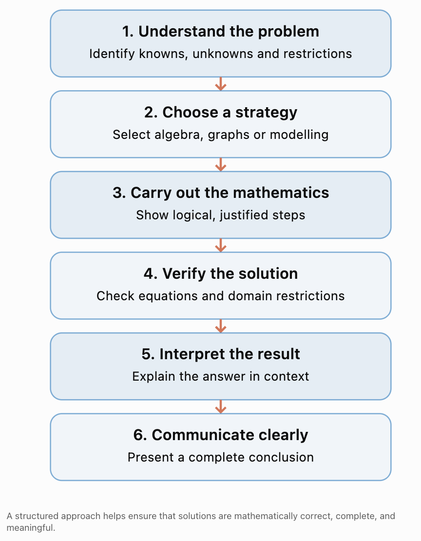
Step 1: Understand the Problem

Before calculating, identify:

• What information is given?

• What quantity must be found?

• Which variables are involved?

• Are there domain restrictions?

• Is an exact or approximate answer required?

• Does the answer need to be interpreted in a real-world context?

Step 2: Select an Appropriate Technique

Different problems suggest different methods.

Step 3: Justify Each Step

A mathematical solution should explain important decisions.

For example:

“We factor the numerator and denominator to identify excluded values and simplify the rational expression.”

This is more informative than simply writing several lines of unexplained algebra.

Step 4: Verify the Answer

Check that solutions:

• Satisfy the original equation.

• Do not make denominators zero.

• Meet any physical restrictions.

• Have appropriate units.

• Are consistent with the graph or model.

Step 5: Communicate the Conclusion

A final answer should state what was found.

Instead of writing only:

x = 80

write:

“The company must produce at least 80 items to achieve the required average cost.”

This makes the mathematical result meaningful.

Connecting the Main Ideas of the Course

Polynomial and rational functions are closely related.

A rational function is formed by dividing one polynomial by another:

f(x) = P(x)/Q(x)

Many rational problems therefore require polynomial techniques.

For example, solving:

requires us to factor the numerator:

(x − 3)(x + 3) = 0

The solutions are x = 3 and x = −3.

However, the domain also requires x ≠ 1.

The same problem involves factoring, solving equations, and checking domain restrictions.

The following sections demonstrate how these skills combine.

Worked Example 1: A Multi-Step Polynomial Equation

Solve:

x⁴ − 5x² + 4 = 0

Step 1: Identify the Structure

This is a fourth-degree polynomial equation, but it contains only even powers of x.

We can use substitution.

Let:

u = x²

Then:

x⁴ = u²

The equation becomes:

u² − 5u + 4 = 0

Step 2: Factor

(u − 1)(u − 4) = 0

Therefore:

u = 1 or u = 4

Step 3: Substitute Back

Since u = x²:

x² = 1 or x² = 4

Taking square roots:

x = ±1 or x = ±2

Step 4: Verify

For x = 2:

2⁴ − 5(2²) + 4

= 16 − 20 + 4

= 0

The other solutions also satisfy the original equation because only even powers appear.

Final answer:

x = −2, −1, 1, 2

Why this method works: Substitution transforms a fourth-degree equation into a quadratic equation that is easier to factor.

Worked Example 2: Factoring a Cubic Polynomial

Solve:

x³ − 4x² − x + 4 = 0

Step 1: Group Terms

(x³ − 4x²) + (−x + 4) = 0

Factor each group:

x²(x − 4) − (x − 4) = 0

Step 2: Factor the Common Binomial

(x − 4)(x² − 1) = 0

Use the difference of squares:

(x − 4)(x − 1)(x + 1) = 0

Step 3: Solve

x − 4 = 0 gives x = 4.

x − 1 = 0 gives x = 1.

x + 1 = 0 gives x = −1.

Final answer:

x = −1, 1, 4

Verification

Substitute x = 4:

64 − 64 − 4 + 4 = 0

Therefore, x = 4 is valid.

The factored form confirms that all three solutions satisfy the equation.

Connection: This problem combines polynomial grouping, the difference-of-squares identity, and the zero-product property.

Worked Example 3: Polynomial Division and the Factor Theorem

A polynomial is given by:

P(x) = 2x³ − 3x² − 11x + 6

Determine whether x − 3 is a factor, and solve P(x) = 0.

Step 1: Apply the Factor Theorem

The factor theorem states:

x − a is a factor of P(x) if P(a) = 0.

Evaluate:

P(3) = 2(27) − 3(9) − 11(3) + 6

= 54 − 27 − 33 + 6

= 0

Therefore, x − 3 is a factor.

Step 2: Divide the Polynomial

Use synthetic division with 3.

Coefficients:

2, −3, −11, 6

The quotient is:

2x² + 3x − 2

Therefore:

P(x) = (x − 3)(2x² + 3x − 2)

Step 3: Factor the Quadratic

2x² + 3x − 2 = (2x − 1)(x + 2)

Therefore:

P(x) = (x − 3)(2x − 1)(x + 2)

Step 4: Solve

x = 3

x = 1/2

x = −2

Final answer:

x = −2, 1/2, 3

Connection: The factor theorem identifies a factor, polynomial division reduces the degree, and quadratic factoring completes the solution.

Worked Example 4: Solving a Rational Equation and Rejecting Extraneous Solutions

Solve:

Step 1: Identify Domain Restrictions

Denominators cannot equal zero.

x − 1 ≠ 0, so x ≠ 1.

x + 1 ≠ 0, so x ≠ −1.

Therefore:

Restrictions: x ≠ 1 and x ≠ −1.

Step 2: Find the Least Common Denominator

The LCD is:

(x − 1)(x + 1)

Multiply every term by the LCD:

(x + 2)(x + 1) = 3(x + 1) + x(x − 1)

Step 3: Expand

Left side:

x² + 3x + 2

Right side:

3x + 3 + x² − x

= x² + 2x + 3

Therefore:

x² + 3x + 2 = x² + 2x + 3

Subtract x² from both sides:

3x + 2 = 2x + 3

x = 1

Step 4: Check the Solution

The algebra produced x = 1.

However, the original equation contains denominators of x − 1.

At x = 1, those denominators become zero.

Therefore, x = 1 is an extraneous solution.

Final answer: No solution.

Why This Happens

Multiplying by an expression containing a variable can produce candidate solutions that do not belong to the original equation's domain.

This is why domain restrictions must be identified before solving and checked afterward.

Worked Example 5: Simplifying a Rational Function with a Hole

Consider:

Determine:

a) The domain.

b) Any holes or vertical asymptotes.

c) The intercepts.

d) The horizontal asymptote.

Step 1: Factor

Numerator:

x² − 4 = (x − 2)(x + 2)

Denominator:

x² − x − 2 = (x − 2)(x + 1)

Therefore:

Step 2: Identify Restrictions

From the original denominator:

x ≠ 2

x ≠ −1

Step 3: Simplify

Cancel the common factor x − 2:

but retain both original restrictions.

Step 4: Identify the Hole

The cancelled factor x − 2 indicates a removable discontinuity at x = 2.

Calculate the corresponding y-value using the simplified expression:

f(2) = (2 + 2)/(2 + 1) = 4/3

Hole: (2, 4/3).

Step 5: Identify the Vertical Asymptote

The remaining denominator is zero when:

x + 1 = 0

x = −1

Vertical asymptote: x = −1.

Step 6: Find Intercepts

For the x-intercept:

x + 2 = 0

x = −2

Therefore:

(−2, 0)

For the y-intercept:

f(0) = 2/1 = 2

Therefore:

(0, 2)

Step 7: Find the Horizontal Asymptote

The simplified numerator and denominator both have degree 1.

The leading coefficient ratio is 1/1.

Horizontal asymptote: y = 1.

Summary

Connection: This problem combines factoring, rational simplification, domain restrictions, discontinuities, intercepts, and asymptotic behaviour.

Worked Example 6: Solving a Rational Inequality

Solve:

Step 1: Identify Critical Values

The numerator equals zero when:

x − 3 = 0

x = 3

The denominator equals zero when:

x + 2 = 0

x = −2

These values divide the number line into three intervals.

Step 2: Test the Intervals

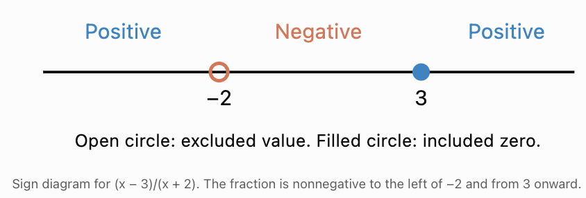
Step 3: Select the Correct Intervals

We require values greater than or equal to zero.

The fraction is positive when x < −2 or x > 3.

At x = 3, the fraction equals zero, so x = 3 is included.

At x = −2, the function is undefined, so x = −2 is excluded.

Final answer:

Why this method works: A rational expression can change sign at zeros of its numerator or denominator. Testing the intervals between these critical values determines where the inequality holds.

Worked Example 7: Complete Analysis of a Rational Function

Analyze:

Determine its domain, intercepts, asymptotes, sign intervals, and end behaviour.

Step 1: Domain

The denominator is zero when x = 1.

Therefore:

Domain: x ≠ 1.

Step 2: Intercepts

Set the numerator equal to zero:

x² − 4 = 0

(x − 2)(x + 2) = 0

x = −2 or x = 2

x-intercepts:

(−2, 0) and (2, 0).

For the y-intercept:

f(0) = (−4)/(−1) = 4

y-intercept:

(0, 4).

Step 3: Vertical Asymptote

At x = 1, the denominator is zero and the numerator is −3, not zero.

Therefore:

Vertical asymptote: x = 1.

Step 4: Oblique Asymptote

The numerator's degree is one greater than the denominator's degree.

Use polynomial division:

As x approaches positive or negative infinity, the final fraction approaches zero.

Therefore:

Oblique asymptote: y = x + 1.

Step 5: Positive and Negative Intervals

Factor the function:

Critical values:

−2, 1, 2.

Test each interval.

Therefore:

Positive: (−2, 1) ∪ (2, ∞).

Negative: (−∞, −2) ∪ (1, 2).

The function equals zero at x = −2 and x = 2.

Step 6: End Behaviour

Because:

f(x) = x + 1 − 3/(x − 1)

the graph approaches y = x + 1 as x becomes large in magnitude.

For large positive x, the graph lies slightly below this line.

For large negative x, it lies slightly above this line.

Step 7: Behaviour Near the Vertical Asymptote

As x approaches 1 from the left:

x − 1 is a small negative number.

−3/(x − 1) becomes very large and positive.

Therefore:

f(x) → +∞.

As x approaches 1 from the right:

−3/(x − 1) becomes very large and negative.

Therefore:

f(x) → −∞.

This information helps us sketch the two branches accurately.

Worked Example 8: Combining Transformations and Graph Features

A function is defined by:

Describe its transformations, domain, range, intercepts, and graph behaviour.

Step 1: Identify the Parent Function

The parent function is:

f(x) = 1/x

Step 2: Identify Transformations

• Reflect in the x-axis.

• Stretch vertically by a factor of 4.

• Translate right 3 units.

• Translate upward 2 units.

Step 3: Domain and Range

Vertical asymptote:

x = 3

Therefore, domain:

x ≠ 3

Horizontal asymptote:

y = 2

Therefore, range:

y ≠ 2

Step 4: x-Intercept

Set g(x) = 0:

−4/(x − 3) + 2 = 0

2 = 4/(x − 3)

2(x − 3) = 4

2x − 6 = 4

x = 5

x-intercept: (5, 0).

Step 5: y-Intercept

g(0) = −4/(−3) + 2

= 4/3 + 2

= 10/3

y-intercept: (0, 10/3).

Step 6: Graph Behaviour

The negative reciprocal coefficient means the branches lie in the upper-left and lower-right regions relative to the asymptote intersection (3, 2).

The function is increasing on both:

(−∞, 3) and (3, ∞).

It is not continuous across x = 3.

Connection: This problem combines function transformations, asymptotes, intercepts, domain, range, and monotonic behaviour.

Worked Example 9: Connecting Polynomial and Rational Models

Two manufacturers have different cost structures.

Company A has total cost:

Cₐ(x) = 400 + 20x

Company B has total cost:

Cᵦ(x) = 700 + 15x

where x is the number of items produced.

Determine which company has the lower average cost.

Step 1: Construct Average-Cost Functions

Average cost = Total cost / Number of items.

For Company A:

A(x) = (400 + 20x)/x

A(x) = 400/x + 20

For Company B:

B(x) = (700 + 15x)/x

B(x) = 700/x + 15

The practical domain is positive whole numbers.

Step 2: Find the Intersection

Set the average costs equal:

400/x + 20 = 700/x + 15

Subtract 15:

400/x + 5 = 700/x

Subtract 400/x:

5 = 300/x

Since x > 0:

5x = 300

x = 60

Step 3: Calculate the Equal Cost

A(60) = 400/60 + 20

≈ $26.67

B(60) = 700/60 + 15

≈ $26.67

Step 4: Compare Other Production Quantities

At 30 items:

A(30) = 400/30 + 20 ≈ $33.33

B(30) = 700/30 + 15 ≈ $38.33

Company A is cheaper.

At 100 items:

A(100) = 400/100 + 20 = $24

B(100) = 700/100 + 15 = $22

Company B is cheaper.

Conclusion

Company A is cheaper for fewer than 60 items.

Both companies have equal average costs at 60 items.

Company B is cheaper for more than 60 items.

Connection: This problem combines linear total-cost models, rational average-cost functions, equation solving, and practical interpretation.

Worked Example 10: Polynomial Optimization

A rectangular garden is built against a wall. The farmer has 100 metres of fencing for the other three sides.

Find the dimensions that maximize the garden's area.

Step 1: Define Variables

Let x be the width perpendicular to the wall.

There are two widths and one fenced length.

Therefore:

2x + L = 100

L = 100 − 2x

Step 2: Construct the Area Function

Area = Length × Width

A(x) = x(100 − 2x)

Expand:

A(x) = −2x² + 100x

Step 3: Determine the Practical Domain

Both dimensions must be positive.

x > 0

100 − 2x > 0

x < 50

Therefore:

0 < x < 50

Step 4: Find the Maximum

The quadratic opens downward.

Its maximum occurs at the vertex:

x = −b/(2a)

x = −100/[2(−2)]

x = 25

Find the length:

L = 100 − 2(25)

L = 50

Step 5: Calculate the Maximum Area

A(25) = 25 × 50

A(25) = 1250 m²

Step 6: Interpret

The garden should be 25 metres wide and 50 metres long.

The maximum area is 1250 m².

The answer is physically valid because both dimensions are positive and the fencing totals 100 metres.

Worked Example 11: Comparing Two Mathematical Models

A company measures the revenue generated by a new product.

Two possible models are proposed:

Linear model:

L(t) = 9t + 8

Quadratic model:

Q(t) = t² + 5t + 10

Determine which model better represents the data.

Step 1: Calculate Predictions

Step 2: Calculate Residuals

Residual = Observed − Predicted.

Linear residuals:

2, −1, −2, −1, 2

Quadratic residuals:

0, 0, 0, 0, 0

Step 3: Calculate Mean Absolute Error

Linear model:

MAE = (2 + 1 + 2 + 1 + 2)/5

MAE = 1.6

Quadratic model:

MAE = 0

Step 4: Evaluate the Models

The quadratic model fits all five observations exactly.

It is therefore the better fit to this dataset.

However, an exact fit does not prove that revenue will continue growing quadratically.

Step 5: Make a Prediction

At t = 5:

Q(5) = 5² + 5(5) + 10

= 25 + 25 + 10

= 60

The model predicts revenue of $60,000 in month 5.

This is an extrapolation because the observed data extend only to month 4.

Conclusion: The quadratic model fits the observations better, but the prediction for month 5 should be treated as an estimate rather than a certainty.

Choosing Efficient Algebraic Strategies

An important part of advanced problem solving is choosing an efficient method.

Consider the following equations.

There is rarely only one possible method. The most efficient approach usually uses the structure of the problem rather than expanding everything immediately.

How to Communicate Mathematical Reasoning Clearly

A complete solution should have four essential parts.

1. Mathematical setup

Define variables and state relevant equations.

2. Logical working

Show enough intermediate steps to make the calculation understandable.

3. Verification

Check the result against the original equation or problem conditions.

4. Conclusion

State the answer with units and context.

Example of an Incomplete Solution

x = 25

A = 1250

Example of a Complete Solution

The garden's area is modelled by:

A(x) = −2x² + 100x

Because the quadratic coefficient is negative, the vertex gives the maximum area.

The vertex occurs at x = 25 metres.

The corresponding length is 50 metres.

Therefore, the maximum area is 1250 m², achieved with dimensions of 25 m by 50 m.

The dimensions satisfy the fencing restriction because:

2(25) + 50 = 100 metres.

The second solution demonstrates the reasoning, verification, and interpretation.

Common Mistakes

Mistake 1: Starting Calculations Without Identifying Restrictions

For rational equations, determine excluded values before multiplying by denominators.

Mistake 2: Cancelling Terms Instead of Factors

Incorrect:

(x + 3)/x = 3

Correct:

(x + 3)/x = 1 + 3/x, for x ≠ 0.

Only common factors can be cancelled.

Mistake 3: Forgetting Extraneous Solutions

Solutions produced after clearing denominators must satisfy the original equation.

Mistake 4: Applying the Zero-Product Property to a Sum

From:

(x − 2)(x + 3) = 0

we can conclude x = 2 or x = −3.

We cannot apply the same rule directly to:

(x − 2) + (x + 3) = 0.

Mistake 5: Using the Wrong Inequality Boundaries

For rational inequalities, both numerator zeros and denominator zeros matter.

Denominator zeros must always be excluded.

Mistake 6: Confusing Holes with Vertical Asymptotes

A factor cancelled from a rational expression may create a hole.

An uncancelled denominator factor may create a vertical asymptote.

Mistake 7: Ignoring Practical Domains

Negative production quantities, impossible dimensions, and times outside a physical event should not be accepted as meaningful answers.

Mistake 8: Assuming a Good Fit Guarantees Accurate Predictions

A model may describe past data well but fail when conditions change.

Mistake 9: Providing Only a Numerical Answer

Complex problems require explanations, verification, and interpretation.

Mistake 10: Choosing an Unnecessarily Complicated Method

Always examine the expression's structure before expanding, dividing, or applying formulas.

Key Terms

• Multi-Step Problem: A problem requiring several connected mathematical operations or techniques.

• Algebraic Strategy: A planned method for solving an equation or analysing a function.

• Polynomial Function: A function formed from nonnegative integer powers of a variable.

• Rational Function: A quotient of two polynomial functions.

• Factor Theorem: A theorem stating that x − a is a factor of P(x) exactly when P(a) = 0.

• Remainder Theorem: A theorem stating that dividing P(x) by x − a gives remainder P(a).

• Synthetic Division: An efficient method of dividing a polynomial by a linear factor of the form x − a.

• Zero-Product Property: If a product equals zero, at least one factor equals zero.

• Extraneous Solution: A candidate solution that does not satisfy the original equation.

• Domain Restriction: A value excluded from a function's domain.

• Removable Discontinuity: A missing point in a graph caused by a removable factor.

• Vertical Asymptote: A vertical line approached as function values become unbounded.

• Oblique Asymptote: A nonhorizontal straight line approached by a graph at infinity.

• Critical Value for Sign Analysis: A zero or excluded input used to divide a number line into sign intervals.

• Optimization: Finding a maximum or minimum under specified conditions.

• Mathematical Model: A mathematical representation of a real-world relationship.

• Residual: Observed value minus predicted value.

• Verification: Checking whether a result satisfies the original conditions.

• Mathematical Justification: Explaining why a mathematical method or conclusion is valid.

• Interpretation: Explaining the meaning of a mathematical result in its context.

Key Takeaways

1. Complex polynomial and rational problems often require several connected techniques.

2. Identifying the structure of an expression helps determine an efficient strategy.

3. Factoring is useful for solving equations, simplifying expressions, and analysing signs.

4. Substitution can simplify certain higher-degree polynomial equations.

5. Rational equations require careful attention to denominator restrictions.

6. Extraneous solutions must be rejected.

7. Rational inequalities are often solved using sign charts.

8. Holes and asymptotes represent different types of discontinuity.

9. Graph transformations help predict function behaviour without extensive calculations.

10. Polynomial and rational functions can be combined to construct real-world models.

11. Optimization problems often involve quadratic functions.

12. Model accuracy should be evaluated using observed data and residuals.

13. Mathematical solutions should include reasoning, verification, and interpretation.

14. The most useful mathematical approach is not always the longest or most complicated one.

Check Your Understanding

These questions combine concepts from throughout the polynomial and rational functions course. Show your working, explain your methods, and verify solutions where appropriate.

Question 1: Polynomial Equations

Solve:

x⁴ − 10x² + 9 = 0

Explain why substitution is an efficient strategy.

Question 2: Factor Theorem and Division

Given:

P(x) = x³ − 2x² − 5x + 6

a) Show that x − 1 is a factor.

b) Factor P(x) completely.

c) Solve P(x) = 0.

Question 3: Rational Equations

Solve:

State domain restrictions and check the result.

Question 4: Rational Simplification

Consider:

a) Factor and simplify.

b) State the domain.

c) Identify any holes and vertical asymptotes.

d) Find the x-intercept.

Question 5: Rational Inequalities

Solve:

Express your answer using interval notation and justify it with sign analysis.

Question 6: Function Transformations

Starting with f(x) = 1/x, a graph is:

• Reflected in the x-axis.

• Stretched vertically by a factor of 2.

• Translated left 3 units.

• Translated upward 4 units.

a) Write its equation.

b) Find its asymptotes.

c) Determine its domain and range.

d) Find its x-intercept.

Question 7: Complete Polynomial Analysis

Analyze:

f(x) = −x² + 8x − 12

Find its intercepts, vertex, range, increasing and decreasing intervals, and positive and negative intervals.

Question 8: Real-World Cost Comparison

Two companies have total-cost models:

C₁(x) = 500 + 12x

C₂(x) = 800 + 9x

where x is the number of products.

a) Write their average-cost functions.

b) Determine the production quantity at which average costs are equal.

c) Determine which company is cheaper at 50 items and at 200 items.

d) Explain your conclusions.

Question 9: Optimization

A rectangular enclosure is built against a wall using 120 metres of fencing for the other three sides.

a) Construct an area function.

b) Determine its practical domain.

c) Find the maximum area.

d) Find the dimensions of the enclosure.

Question 10: Integrated Challenge

A function is given by:

a) Find its domain.

b) Find its x- and y-intercepts.

c) Find its vertical asymptote.

d) Use polynomial division to determine its oblique asymptote.

e) Determine where the function is positive and negative.

f) Describe its behaviour near the vertical asymptote.

g) Explain how the results help construct an accurate graph.

Fully Worked Answers

Answer 1: Polynomial Equations

Given:

x⁴ − 10x² + 9 = 0

Let:

u = x²

Then:

u² − 10u + 9 = 0

Factor:

(u − 1)(u − 9) = 0

Therefore:

u = 1 or u = 9

Substitute back:

x² = 1 or x² = 9

Therefore:

x = −3, −1, 1, 3.

Substitution is efficient because it converts a fourth-degree equation into a quadratic equation.

All four values satisfy the original equation.

Answer 2: Factor Theorem

Given:

P(x) = x³ − 2x² − 5x + 6

a) Verify x − 1 is a factor.

Evaluate P(1):

P(1) = 1 − 2 − 5 + 6 = 0

Therefore, x − 1 is a factor.

b) Factor completely.

Divide P(x) by x − 1.

The quotient is:

x² − x − 6

Factor:

x² − x − 6 = (x − 3)(x + 2)

Therefore:

P(x) = (x − 1)(x − 3)(x + 2)

c) Solve.

Set each factor equal to zero:

x = 1, 3, −2

Final answer: x = −2, 1, 3.

Answer 3: Rational Equation

Given:

Step 1: Domain restriction

x ≠ 2.

Step 2: Multiply by x − 2.

x + 3 = 5 + 2(x − 2)

Expand:

x + 3 = 5 + 2x − 4

x + 3 = 2x + 1

x = 2

Step 3: Verify

But x = 2 makes the original denominators zero.

Therefore, the candidate is extraneous.

Final answer: No solution.

Answer 4: Rational Simplification

Given:

a) Factor.

Numerator:

(x − 3)(x + 3)

Denominator:

(x − 3)(x + 1)

Therefore:

with the original restrictions retained.

b) Domain

x ≠ 3 and x ≠ −1.

c) Hole and vertical asymptote

The cancelled factor x − 3 produces a hole at x = 3.

Its y-coordinate is:

(3 + 3)/(3 + 1) = 6/4 = 3/2

Hole: (3, 3/2).

The remaining denominator gives:

Vertical asymptote: x = −1.

d) x-intercept

x + 3 = 0

x = −3

Therefore:

x-intercept: (−3, 0).

Answer 5: Rational Inequality

Given:

Critical values:

x = −1 and x = 4.

Test the intervals.

For x < −1, both numerator and denominator are negative, giving a positive fraction.

For −1 < x < 4, the numerator is positive and denominator negative, giving a negative fraction.

For x > 4, both are positive, giving a positive fraction.

The inequality requires a strictly negative result.

Therefore:

Neither endpoint is included.

At x = −1, the expression equals zero.

At x = 4, it is undefined.

Answer 6: Function Transformations

Original:

f(x) = 1/x

a) Equation

Reflect and stretch:

−2/x

Translate left 3:

−2/(x + 3)

Translate up 4:

b) Asymptotes

Vertical: x = −3.

Horizontal: y = 4.

c) Domain and range

Domain: x ≠ −3.

Range: y ≠ 4.

d) x-intercept

Set g(x) = 0:

−2/(x + 3) + 4 = 0

4 = 2/(x + 3)

4(x + 3) = 2

4x + 12 = 2

4x = −10

x = −5/2

x-intercept: (−5/2, 0).

Answer 7: Complete Polynomial Analysis

Given:

f(x) = −x² + 8x − 12

Intercepts

Set f(x) = 0:

−x² + 8x − 12 = 0

Multiply by −1:

x² − 8x + 12 = 0

(x − 2)(x − 6) = 0

x = 2 or x = 6

x-intercepts:

(2, 0), (6, 0).

y-intercept:

f(0) = −12

Therefore:

(0, −12).

Vertex

x = −8/[2(−1)] = 4

f(4) = −16 + 32 − 12 = 4

Vertex: (4, 4).

This is a maximum because the parabola opens downward.

Range

y ≤ 4.

Increasing and decreasing

Increasing: (−∞, 4).

Decreasing: (4, ∞).

Positive and negative

Positive: (2, 6).

Negative: (−∞, 2) ∪ (6, ∞).

Answer 8: Cost Comparison

Given:

C₁(x) = 500 + 12x

C₂(x) = 800 + 9x

a) Average-cost functions

A₁(x) = 500/x + 12

A₂(x) = 800/x + 9

b) Equal average costs

500/x + 12 = 800/x + 9

3 = 300/x

3x = 300

x = 100

At 100 items, both average costs are:

500/100 + 12 = $17

800/100 + 9 = $17

c) At 50 items

A₁(50) = 500/50 + 12 = $22

A₂(50) = 800/50 + 9 = $25

Company 1 is cheaper.

At 200 items:

A₁(200) = 500/200 + 12 = $14.50

A₂(200) = 800/200 + 9 = $13

Company 2 is cheaper.

d) Interpretation

Company 1 has lower fixed costs.

Company 2 has lower variable costs.

Company 1 is preferable at lower production quantities, while Company 2 becomes preferable above 100 items.

Answer 9: Optimization

Let x represent the width perpendicular to the wall.

Two widths and one length require 120 metres of fencing.

2x + L = 120

Therefore:

L = 120 − 2x

a) Area function

A(x) = x(120 − 2x)

A(x) = −2x² + 120x

b) Practical domain

x > 0

120 − 2x > 0

x < 60

Therefore:

0 < x < 60

c) Maximum area

Vertex:

x = −120/[2(−2)]

x = 30

Length:

120 − 2(30) = 60

Maximum area:

A(30) = 30 × 60 = 1800 m²

d) Dimensions

Width: 30 m.

Length: 60 m.

The fencing requirement is satisfied:

2(30) + 60 = 120 m.

Answer 10: Integrated Challenge

Given:

a) Domain

Denominator cannot equal zero.

x − 4 ≠ 0

Therefore:

x ≠ 4.

b) Intercepts

Factor numerator:

x² − x − 6 = (x − 3)(x + 2)

x-intercepts:

x = 3 and x = −2

Therefore:

(3, 0) and (−2, 0).

y-intercept:

f(0) = −6/(−4) = 3/2

Therefore:

(0, 3/2).

c) Vertical asymptote

x = 4.

The numerator at x = 4 is:

16 − 4 − 6 = 6

Since the numerator is nonzero, x = 4 is a vertical asymptote.

d) Oblique asymptote

Divide x² − x − 6 by x − 4.

The quotient is x + 3, with remainder 6.

Therefore:

As x becomes large in magnitude, 6/(x − 4) approaches zero.

Oblique asymptote:

y = x + 3.

e) Positive and negative intervals

Factor:

Critical values:

−2, 3, 4.

Test intervals.

Therefore:

Positive: (−2, 3) ∪ (4, ∞).

Negative: (−∞, −2) ∪ (3, 4).

f) Behaviour near the vertical asymptote

Use:

f(x) = x + 3 + 6/(x − 4)

As x approaches 4 from the left:

6/(x − 4) → −∞

Therefore:

f(x) → −∞.

As x approaches 4 from the right:

6/(x − 4) → +∞

Therefore:

f(x) → +∞.

g) Constructing the graph

An accurate sketch should show:

• x-intercepts at (−2, 0) and (3, 0).

• y-intercept at (0, 3/2).

• Vertical asymptote x = 4.

• Oblique asymptote y = x + 3.

• A left branch approaching negative infinity as x approaches 4 from below.

• A right branch approaching positive infinity as x approaches 4 from above.

• Both branches approaching y = x + 3 for large magnitudes of x.

These features allow us to sketch the graph without constructing a large table of values.

Final Course Connections

The study of polynomial and rational functions is built around several closely related ideas.

Algebraic structure helps us simplify expressions and solve equations.

Function behaviour helps us understand intercepts, turning points, discontinuities, asymptotes, and end behaviour.

Transformations allow us to predict graphs from familiar parent functions.

Mathematical modelling connects these functions to real-world situations.

Verification and communication ensure that solutions are valid, understandable, and meaningful.

The strongest problem solvers do not simply memorize methods. They recognize mathematical structures, choose suitable strategies, connect ideas, and explain why their conclusions are justified.

This completes Comprehensive Problem Solving, bringing together the major concepts and skills developed throughout the polynomial and rational functions course.