Applications and Function Analysis

Introduction

Functions are used to describe patterns, relationships, and changes in the world around us. Once we understand the graph of a basic function, we can create many new graphs by shifting, reflecting, stretching, or compressing it.

These changes are called function transformations.

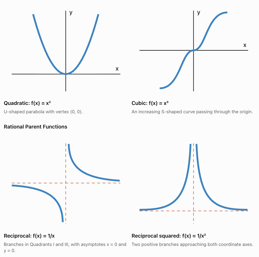
For example, the basic quadratic function:

f(x) = x²

produces a parabola with its vertex at the origin.

By changing its equation to:

g(x) = (x − 3)² + 2

we move the parabola 3 units to the right and 2 units upward.

The shape remains the same, but its position changes.

Function transformations are especially useful because they allow us to predict the shape and location of a graph without plotting large numbers of points.

The same transformation principles apply to polynomial functions, rational functions, exponential functions, and many other families.

In this lesson, we will review how transformations affect polynomial and rational functions, predict graph changes from equations, write transformed equations, and sketch graphs using key features.

Understanding Parent Functions

A parent function is a basic function from which other related functions can be produced through transformations.

Common parent functions include:

In this lesson, we focus mainly on polynomial and rational parent functions.

Polynomial Parent Functions

The General Transformation Equation

Many transformed functions can be written as:

where:

• a controls vertical stretching, compression, and reflection in the x-axis.

• b controls horizontal stretching, compression, and reflection in the y-axis.

• h controls horizontal translation.

• k controls vertical translation.

These parameters affect the graph in predictable ways.

Important: Horizontal transformations work in the opposite direction from what the sign inside the brackets might initially suggest.

For example:

f(x − 4) moves the graph right 4 units, not left.

Vertical Translations

A vertical translation moves every point on a graph up or down.

If:

g(x) = f(x) + k

then every output increases by k.

The point (x, y) becomes:

(x, y + k)

Worked Example 1: Vertical Translation of a Polynomial

Consider:

f(x) = x²

Translate the graph upward 5 units.

The new equation is:

g(x) = x² + 5

The vertex moves from (0, 0) to (0, 5).

The domain remains all real numbers.

The range changes from y ≥ 0 to y ≥ 5.

Worked Example 2: Vertical Translation of a Rational Function

Consider:

f(x) = 1/x

Translate the graph downward 3 units.

The new equation is:

g(x) = 1/x − 3

The vertical asymptote remains:

x = 0

The horizontal asymptote moves from y = 0 to:

y = −3

The domain remains x ≠ 0.

The range becomes y ≠ −3.

Horizontal Translations

A horizontal translation moves a graph left or right.

If:

g(x) = f(x − h)

the graph moves right h units when h is positive.

If:

g(x) = f(x + h)

the graph moves left h units when h is positive.

Worked Example 3: Horizontal Translation of a Quadratic

Consider:

f(x) = x²

Translate the graph right 4 units.

The new equation is:

g(x) = (x − 4)²

The vertex moves from (0, 0) to (4, 0).

The axis of symmetry becomes:

x = 4

Worked Example 4: Horizontal Translation of a Rational Function

Consider:

f(x) = 1/x

Translate the graph left 2 units.

The new equation is:

g(x) = 1/(x + 2)

The vertical asymptote moves from x = 0 to:

x = −2

The horizontal asymptote remains y = 0.

The domain becomes x ≠ −2.

Reflections

Reflections produce mirror images of graphs.

Reflection in the x-Axis

To reflect a function in the x-axis:

g(x) = −f(x)

Every output changes sign.

A point (x, y) becomes:

(x, −y)

Worked Example 5: Reflecting a Quadratic

Original:

f(x) = x²

Reflected:

g(x) = −x²

The parabola changes from opening upward to opening downward.

The vertex remains at (0, 0).

The range changes from y ≥ 0 to y ≤ 0.

Reflection in the y-Axis

To reflect a function in the y-axis:

g(x) = f(−x)

A point (x, y) becomes:

(−x, y)

Worked Example 6: Reflecting a Cubic

Original:

f(x) = x³

Reflected:

g(x) = (−x)³

Therefore:

g(x) = −x³

The graph changes from increasing to decreasing.

Symmetry and Reflections

Some functions remain unchanged under certain reflections.

For example:

f(x) = x²

Then:

f(−x) = (−x)² = x²

The graph is symmetric about the y-axis.

Such functions are called even functions.

For:

f(x) = x³

f(−x) = −x³ = −f(x)

This function is symmetric about the origin and is called an odd function.

These symmetry properties can make some transformations appear to have the same effect.

Vertical Stretches and Compressions

A vertical stretch or compression changes the distance of each point from the x-axis.

For:

g(x) = af(x)

the output values are multiplied by a.

• If |a| > 1, the graph is stretched vertically.

• If 0 < |a| < 1, the graph is compressed vertically.

• If a < 0, the graph is also reflected in the x-axis.

Worked Example 7: Stretching a Quadratic

Original function:

f(x) = x²

Apply a vertical stretch by a factor of 3.

New equation:

g(x) = 3x²

Compare the outputs:

The transformed parabola appears narrower because its outputs increase more quickly as x moves away from zero.

The vertex remains at (0, 0).

Worked Example 8: Compressing a Rational Function

Original:

f(x) = 1/x

Apply a vertical compression by a factor of 1/2.

New equation:

g(x) = 1/(2x)

Every output is half its original value.

For example:

f(2) = 1/2

g(2) = 1/4

The asymptotes remain x = 0 and y = 0.

The branches move closer to the x-axis for corresponding x-values.

Horizontal Stretches and Compressions

Horizontal transformations change the x-coordinates of points.

For:

g(x) = f(bx)

the x-coordinates are divided by b, provided b ≠ 0.

If b = 2, the graph is compressed horizontally by a factor of 1/2.

If b = 1/3, the graph is stretched horizontally by a factor of 3.

Worked Example 9: Horizontal Compression of a Cubic

Original:

f(x) = x³

Apply a horizontal compression by a factor of 1/2.

New equation:

g(x) = f(2x)

Therefore:

g(x) = (2x)³ = 8x³

The original point (2, 8) moves to (1, 8).

Although the equation resembles a vertical stretch by a factor of 8, the specified transformation was a horizontal compression.

Important: Different transformations can sometimes produce the same final equation, particularly for power functions.

Worked Example 10: Horizontal Stretch of a Rational Function

Original:

f(x) = 1/(x − 1)

Apply a horizontal stretch by a factor of 2.

New equation:

g(x) = f(x/2)

Substitute x/2 for x:

Multiply numerator and denominator by 2:

The original vertical asymptote x = 1 moves to x = 2.

The horizontal asymptote remains y = 0.

Combining Transformations

Most transformed functions involve more than one transformation.

The general equation is:

g(x) = af(b(x − h)) + k

A point (u, v) on the original graph transforms to:

This coordinate rule is particularly useful for accurate sketching.

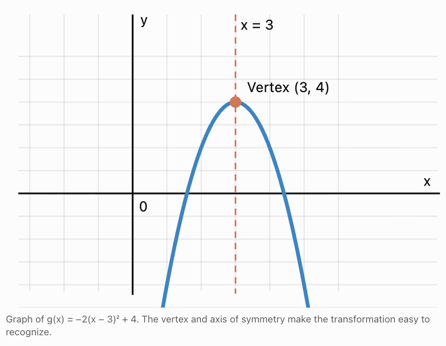
Worked Example 11: Transforming a Quadratic Function

Starting with:

f(x) = x²

Apply the following transformations:

1. Reflect in the x-axis.

2. Stretch vertically by a factor of 2.

3. Translate right 3 units.

4. Translate upward 4 units.

Step 1: Reflection and vertical stretch.

−2x²

Step 2: Horizontal translation.

−2(x − 3)²

Step 3: Vertical translation.

The vertex is (3, 4).

The parabola opens downward.

The maximum value is 4.

The axis of symmetry is x = 3.

The domain is all real numbers.

The range is y ≤ 4.

Sketching the Transformed Quadratic

Worked Example 12: Transforming a Rational Function

Starting with:

f(x) = 1/x

Apply the following transformations:

1. Reflect in the x-axis.

2. Stretch vertically by a factor of 3.

3. Translate right 2 units.

4. Translate upward 1 unit.

The resulting equation is:

Vertical asymptote:

x = 2

Horizontal asymptote:

y = 1

Domain:

x ≠ 2

Range:

y ≠ 1

x-intercept:

Set g(x) = 0:

−3/(x − 2) + 1 = 0

3/(x − 2) = 1

x − 2 = 3

x = 5

Therefore, (5, 0).

y-intercept:

g(0) = −3/(−2) + 1

= 3/2 + 1

= 5/2

Therefore, (0, 2.5).

The negative coefficient reverses the orientation of the reciprocal branches. For x less than 2, the graph lies above y = 1. For x greater than 2, it lies below y = 1.

Predicting Graph Changes from Equations

One of the most useful transformation skills is identifying graph changes without plotting points.

Worked Example 13: Interpreting a Polynomial Equation

Consider:

g(x) = 4(x + 2)² − 3

Compare this with:

f(x) = x²

We can identify:

• A vertical stretch by a factor of 4.

• A translation left 2 units.

• A translation down 3 units.

• No reflection.

The vertex is (−2, −3).

The parabola opens upward.

The range is y ≥ −3.

Worked Example 14: Interpreting a Rational Equation

Consider:

g(x) = 2/(x + 4) − 5

Compare with:

f(x) = 1/x

We can identify:

• A vertical stretch by a factor of 2.

• A translation left 4 units.

• A translation down 5 units.

The vertical asymptote is x = −4.

The horizontal asymptote is y = −5.

The domain excludes x = −4.

The range excludes y = −5.

Worked Example 15: Interpreting a Horizontal Reflection

Consider:

g(x) = (−x + 3)³

Rewrite:

g(x) = [−(x − 3)]³

Starting with f(x) = x³, this represents a reflection in the y-axis followed by a translation right 3 units.

Because the cubic parent function is odd:

g(x) = −(x − 3)³

Therefore, it can also be described as a reflection in the x-axis followed by a translation right 3 units.

The inflection point is (3, 0).

This example demonstrates that the same transformed graph can sometimes be produced by different sequences of transformations.

Writing Equations from Graph Features

We can reverse the transformation process.

Instead of starting with an equation and identifying changes, we use the graph's features to construct an equation.

Worked Example 16: Writing a Quadratic Equation

A parabola has:

• Vertex (4, −2).

• Opens upward.

• Passes through (5, 1).

Write its equation.

Step 1: Use vertex form.

g(x) = a(x − h)² + k

Substitute the vertex:

g(x) = a(x − 4)² − 2

Step 2: Substitute the known point.

1 = a(5 − 4)² − 2

1 = a − 2

a = 3

Final equation:

Worked Example 17: Writing a Rational Function

A transformed reciprocal graph has:

• Vertical asymptote x = 3.

• Horizontal asymptote y = −2.

• Passes through (4, 1).

Write its equation.

Step 1: Use transformed reciprocal form.

g(x) = a/(x − h) + k

Step 2: Substitute the asymptotes.

h = 3 and k = −2.

Therefore:

g(x) = a/(x − 3) − 2

Step 3: Substitute the known point.

1 = a/(4 − 3) − 2

1 = a − 2

a = 3

Final equation:

This is a vertical stretch by a factor of 3, followed by a translation right 3 units and down 2 units.

Sketching Transformed Graphs Accurately

A good sketch should show the function's defining features rather than rely on many randomly selected points.

Sketching Polynomial Transformations

For a quadratic function:

g(x) = a(x − h)² + k

1. Identify the vertex (h, k).

2. Determine whether the parabola opens upward or downward.

3. Use |a| to determine its vertical stretch or compression.

4. Draw the axis of symmetry x = h.

5. Plot points on both sides of the vertex.

6. Connect the points with a smooth curve.

Worked Example 18: Sketching a Transformed Quadratic

Sketch:

g(x) = 2(x + 1)² − 3

The vertex is (−1, −3).

The parabola opens upward.

It is stretched vertically by a factor of 2.

The axis of symmetry is x = −1.

Calculate points:

Plot these points and connect them with a smooth U-shaped curve.

Sketching Rational Transformations

For a transformed reciprocal function:

g(x) = a/(x − h) + k

1. Identify the vertical asymptote x = h.

2. Identify the horizontal asymptote y = k.

3. Draw both asymptotes as dashed lines.

4. Determine the sign of a.

5. Plot points on both sides of the vertical asymptote.

6. Sketch the branches approaching the asymptotes.

For a > 0, the branches lie in the upper-right and lower-left regions relative to the asymptote intersection (h, k).

For a < 0, the branches lie in the upper-left and lower-right regions.

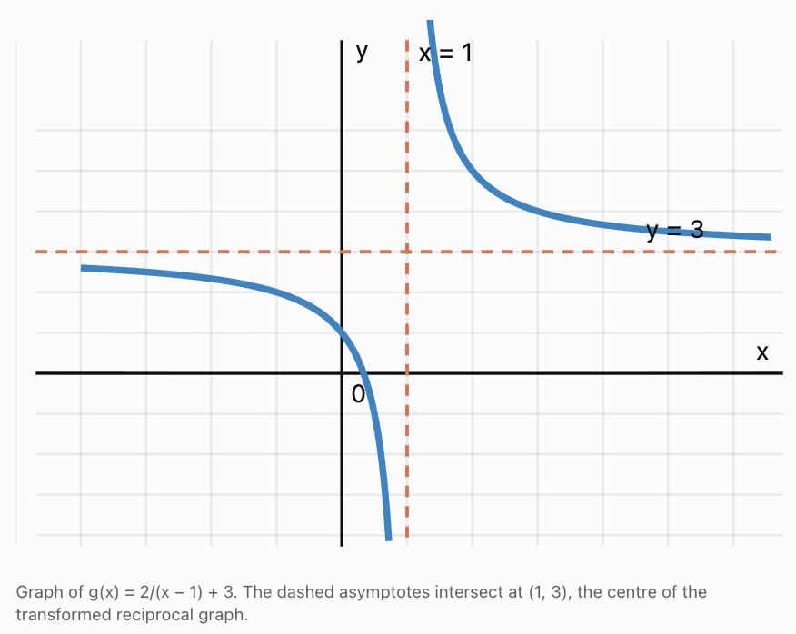
Worked Example 19: Sketching a Transformed Rational Function

Sketch:

g(x) = 2/(x − 1) + 3

Step 1: Identify asymptotes.

Vertical asymptote: x = 1.

Horizontal asymptote: y = 3.

Step 2: Determine orientation.

The coefficient 2 is positive.

The right branch lies above y = 3.

The left branch lies below y = 3.

Step 3: Calculate points.

How Transformations Affect Domain, Range, and Asymptotes

Transformations can change more than the appearance of a graph.

They may also change the domain, range, intercepts, extrema, and asymptotes.

Polynomial Functions

For:

g(x) = a(x − h)² + k

with a ≠ 0:

• Domain: all real numbers.

• Vertex: (h, k).

• Axis of symmetry: x = h.

• Range: y ≥ k if a > 0.

• Range: y ≤ k if a < 0.

Rational Functions

For:

g(x) = a/(x − h) + k

with a ≠ 0:

• Domain: x ≠ h.

• Range: y ≠ k.

• Vertical asymptote: x = h.

• Horizontal asymptote: y = k.

These formulas allow us to predict major graph features immediately.

Real-World Applications

Application 1: Projectile Motion

A ball's height is modelled by:

h(t) = −5(t − 3)² + 47

This is a transformed quadratic function.

Compared with f(t) = t², it has been:

• Reflected in the horizontal axis.

• Stretched vertically by a factor of 5.

• Translated right 3 units.

• Translated upward 47 units.

The vertex is (3, 47).

Interpretation: The ball reaches a maximum height of 47 metres after 3 seconds.

The negative coefficient represents the downward curvature caused by gravity.

The physical model is relevant only over the time interval during which the ball is in flight.

Application 2: Average Production Cost

A company models its average cost per item using:

A(x) = 500/x + 20

This is a transformed reciprocal function.

Compared with f(x) = 1/x:

• It has been stretched vertically by a factor of 500.

• It has been translated upward 20 units.

The horizontal asymptote is y = 20.

Interpretation: As production increases, average cost approaches $20 per item.

The vertical asymptote is x = 0, but the practical domain is positive whole-number production quantities.

Application 3: Modelling a Parabolic Arch

An arch is modelled by:

h(x) = −0.25(x − 4)² + 6

where h is height in metres and x is horizontal distance.

The vertex is (4, 6).

The arch reaches a maximum height of 6 metres at x = 4.

To find where it meets ground level, set h(x) = 0:

−0.25(x − 4)² + 6 = 0

0.25(x − 4)² = 6

(x − 4)² = 24

x = 4 ± √24

Approximately:

x ≈ −0.90 and x ≈ 8.90

The arch spans approximately 9.80 metres between its ground-level intercepts.

Application 4: Temperature Adjustment

Suppose a temperature model is:

T(t) = 15 + 10 sin(t)

If a new environment is consistently 5 degrees warmer, the transformed model becomes:

T₂(t) = T(t) + 5

Therefore:

T₂(t) = 20 + 10 sin(t)

This is a vertical translation upward by 5 units.

The maximum and minimum temperatures both increase by 5, while the timing of those extrema remains unchanged.

This demonstrates that transformation principles apply beyond polynomial and rational functions.

Common Mistakes

Mistake 1: Reversing Horizontal Translations

Incorrect: f(x − 3) moves left 3 units.

Correct: f(x − 3) moves right 3 units.

Mistake 2: Confusing Vertical and Horizontal Stretching

The expression 3f(x) represents a vertical stretch by a factor of 3.

The expression f(3x) represents a horizontal compression by a factor of 1/3.

Mistake 3: Forgetting Reflections

A negative coefficient outside the function reflects the graph in the x-axis.

A negative multiplier on the input reflects it in the y-axis.

Mistake 4: Incorrectly Transforming Rational Asymptotes

For g(x) = 1/(x − 4) + 2:

The vertical asymptote is x = 4, not x = −4.

The horizontal asymptote is y = 2, not y = −2.

Mistake 5: Applying Only One Transformation

For g(x) = −3(x + 2)² + 5, the graph is reflected, stretched, shifted left, and shifted upward.

All transformations must be considered.

Mistake 6: Ignoring Domain Restrictions

For rational functions, excluded values must be preserved.

A transformation may move a vertical asymptote or hole to a new location.

Mistake 7: Sketching Without Key Features

For a quadratic, identify the vertex and axis of symmetry first.

For a reciprocal function, identify the asymptotes and branch orientation first.

Mistake 8: Assuming Transformations Always Change the Graph Uniquely

Some transformations produce identical results because of symmetry or algebraic identities.

For example, reflecting y = x² in the y-axis does not change its graph.

Key Terms

• Parent Function: A basic function used as the starting point for transformations.

• Transformation: A change in the position, orientation, or scale of a graph.

• Translation: A shift of a graph without changing its shape.

• Vertical Translation: Moving a graph upward or downward.

• Horizontal Translation: Moving a graph left or right.

• Reflection: Producing a mirror image of a graph across a line.

• Vertical Stretch: Multiplying outputs by a factor greater than 1 in magnitude.

• Vertical Compression: Multiplying outputs by a positive factor less than 1.

• Horizontal Stretch: Increasing horizontal distances by a scale factor.

• Horizontal Compression: Decreasing horizontal distances by a scale factor.

• Vertex: The turning point of a parabola.

• Axis of Symmetry: A line dividing a graph into mirror-image halves.

• Asymptote: A line that a graph approaches in a particular limiting situation.

• Vertical Asymptote: A vertical line approached by a graph as outputs become unbounded.

• Horizontal Asymptote: A horizontal line approached as x tends toward infinity or negative infinity.

• Domain: The set of permitted input values.

• Range: The set of possible output values.

• Even Function: A function satisfying f(−x) = f(x).

• Odd Function: A function satisfying f(−x) = −f(x).

• Transformed Equation: An equation produced by applying transformations to a parent function.

Key Takeaways

1. Function transformations allow us to predict new graphs from known parent functions.

2. Adding a constant outside a function moves its graph vertically.

3. Changing the input to x − h moves a graph right h units.

4. Multiplying a function by a negative number reflects it in the x-axis.

5. Replacing x with −x reflects a graph in the y-axis.

6. Vertical stretches and compressions multiply the output values.

7. Horizontal stretches and compressions change the input scale.

8. The general transformation form is g(x) = af(b(x − h)) + k.

9. For a transformed quadratic, the vertex is a key feature for sketching.

10. For a transformed reciprocal function, the asymptotes are key features for sketching.

11. Transformations can change intercepts, extrema, domain restrictions, ranges, and asymptotes.

12. The same transformation rules apply to polynomial, rational, and many other function families.

13. Accurate sketches should include key coordinates, appropriate symmetry, and asymptotes where necessary.

Check Your Understanding

Question 1: Vertical and Horizontal Translations

Starting with f(x) = x², write the equation after translating:

a) Right 4 units.

b) Left 2 units and up 5 units.

c) Right 3 units and down 6 units.

Question 2: Reflections

Starting with f(x) = x³, write the equation after:

a) Reflection in the x-axis.

b) Reflection in the y-axis.

c) Reflection in both axes.

Question 3: Vertical Stretches and Compressions

Starting with f(x) = x², write the equation after:

a) A vertical stretch by a factor of 4.

b) A vertical compression by a factor of 1/3.

c) Reflection in the x-axis followed by a vertical stretch by a factor of 2.

Question 4: Interpreting a Transformed Quadratic

Consider:

g(x) = −3(x − 2)² + 7

Identify:

a) Parent function.

b) Transformations.

c) Vertex.

d) Axis of symmetry.

e) Domain and range.

Question 5: Transforming a Rational Function

Starting with f(x) = 1/x, apply:

• Translation right 5 units.

• Translation downward 2 units.

• Vertical stretch by a factor of 3.

Write the equation and identify its asymptotes.

Question 6: Writing an Equation from a Vertex

A parabola has vertex (−3, 4), opens upward, and passes through (−2, 6).

Write its equation in vertex form.

Question 7: Writing a Rational Function

A reciprocal graph has:

• Vertical asymptote x = −2.

• Horizontal asymptote y = 4.

• Passes through (−1, 7).

Find its equation.

Question 8: Sketching a Transformed Quadratic

Sketch:

g(x) = (x − 1)² − 4

Identify the vertex, axis of symmetry, intercepts, and range.

Question 9: Sketching a Transformed Rational Function

Sketch:

g(x) = −2/(x + 1) + 3

Identify the domain, range, asymptotes, intercepts, and branch orientation.

Question 10: Challenge — Combined Transformations

Starting with:

f(x) = x³

Apply the following transformations:

• Reflect in the x-axis.

• Compress horizontally by a factor of 1/2.

• Translate right 2 units.

• Translate upward 5 units.

Write the final equation and determine the transformed location of the parent function's origin.

Fully Worked Answers

Answer 1: Translations

a) Right 4 units:

g(x) = (x − 4)²

b) Left 2 and up 5:

g(x) = (x + 2)² + 5

c) Right 3 and down 6:

g(x) = (x − 3)² − 6

Answer 2: Reflections

Original:

f(x) = x³

a) Reflection in x-axis:

g(x) = −x³

b) Reflection in y-axis:

g(x) = (−x)³ = −x³

c) Reflection in both axes:

g(x) = −(−x)³ = x³

The original graph is recovered because the two reflections cancel for this odd function.

Answer 3: Vertical Scaling

a) Vertical stretch by 4:

g(x) = 4x²

b) Vertical compression by 1/3:

g(x) = (1/3)x²

c) Reflection and vertical stretch by 2:

g(x) = −2x²

Answer 4: Transformed Quadratic

Given:

g(x) = −3(x − 2)² + 7

a) Parent function:

f(x) = x²

b) Transformations:

Reflection in x-axis, vertical stretch by factor 3, translation right 2, and translation up 7.

c) Vertex:

(2, 7)

d) Axis of symmetry:

x = 2

e) Domain and range:

Domain: all real numbers.

Range: y ≤ 7.

Answer 5: Rational Transformation

Original:

f(x) = 1/x

Right 5 units:

1/(x − 5)

Vertical stretch by 3:

3/(x − 5)

Down 2 units:

Vertical asymptote:

x = 5

Horizontal asymptote:

y = −2

Answer 6: Quadratic Equation from Vertex

Vertex:

(−3, 4)

Use vertex form:

g(x) = a(x + 3)² + 4

Substitute point (−2, 6):

6 = a(−2 + 3)² + 4

6 = a + 4

a = 2

Final equation:

g(x) = 2(x + 3)² + 4

Answer 7: Rational Equation from Asymptotes

Vertical asymptote:

x = −2

Horizontal asymptote:

y = 4

Use:

g(x) = a/(x + 2) + 4

Substitute point (−1, 7):

7 = a/(−1 + 2) + 4

7 = a + 4

a = 3

Final equation:

g(x) = 3/(x + 2) + 4

Answer 8: Quadratic Sketch

Given:

g(x) = (x − 1)² − 4

Vertex:

(1, −4)

Axis of symmetry:

x = 1

x-intercepts:

Set g(x) = 0:

(x − 1)² − 4 = 0

(x − 1)² = 4

x − 1 = ±2

x = −1 or x = 3

Therefore:

(−1, 0) and (3, 0).

y-intercept:

g(0) = (−1)² − 4 = −3

Therefore:

(0, −3).

Range:

y ≥ −4.

Sketch an upward-opening parabola through these points, symmetric about x = 1.

Answer 9: Rational Sketch

Given:

g(x) = −2/(x + 1) + 3

Domain:

x ≠ −1.

Range:

y ≠ 3.

Vertical asymptote:

x = −1.

Horizontal asymptote:

y = 3.

x-intercept:

Set g(x) = 0:

−2/(x + 1) + 3 = 0

3 = 2/(x + 1)

3(x + 1) = 2

3x + 3 = 2

x = −1/3

Therefore:

(−1/3, 0).

y-intercept:

g(0) = −2/1 + 3 = 1

Therefore:

(0, 1).

Branch orientation:

Because the coefficient is negative, the left branch lies above y = 3 and the right branch lies below y = 3.

Answer 10: Combined Transformations

Original:

f(x) = x³

Step 1: Reflect in the x-axis.

−x³

Step 2: Compress horizontally by factor 1/2.

Replace x with 2x:

−(2x)³

Step 3: Translate right 2 units.

−[2(x − 2)]³

Step 4: Translate upward 5 units.

Simplify:

The origin (0, 0) of the parent graph moves to (2, 5).

This is the transformed cubic's inflection point.

Final equation: g(x) = −8(x − 2)³ + 5.

This completes Function Transformations Review, covering polynomial and rational transformations, predicting graph changes, writing equations, accurate sketching, and real-world applications.