5. The Remainder and Factor Theorems

The Remainder and Factor Theorems

Introduction

The Remainder Theorem and Factor Theorem are powerful algebraic tools that connect polynomial division, substitution, factoring, and solving equations.

These theorems allow us to answer important questions without performing lengthy polynomial division.

For example, suppose we have:

P(x) = x³ − 4x² + x + 6

We might want to know:

• What is the remainder when P(x) is divided by x − 2?

• Is x − 3 a factor of P(x)?

• Can we find the zeros of the polynomial?

• How can we evaluate a polynomial efficiently?

• How are polynomial factors connected to its graph?

The Remainder and Factor Theorems provide efficient methods for answering these questions.

They are especially useful when working with quadratic, cubic, and higher-degree polynomials.

Review: Polynomial Division

When one polynomial is divided by another, the result can be expressed using a quotient and remainder.

The general relationship is:

P(x) = D(x)Q(x) + R(x)

Where:

• P(x) is the dividend.

• D(x) is the divisor.

• Q(x) is the quotient.

• R(x) is the remainder.

The remainder must have a degree lower than the divisor, unless the remainder is zero.

Example

Suppose:

P(x) = x² + 5x + 7

Divide by:

D(x) = x + 2

The quotient is:

Q(x) = x + 3

The remainder is:

R = 1

Therefore:

x² + 5x + 7 = (x + 2)(x + 3) + 1

This relationship is the foundation of the Remainder Theorem.

The Remainder Theorem

The Remainder Theorem states:

When a polynomial P(x) is divided by x − a, the remainder is equal to P(a).

In symbols:

Remainder = P(a)

This means we can calculate the remainder simply by substituting a value into the polynomial.

We do not need to perform polynomial long division.

Important Sign Rule

The value used is the number that makes the divisor equal to zero.

Applying the Remainder Theorem

Worked Example

Find the remainder when:

P(x) = x² + 3x + 5

is divided by:

x − 2

Step 1: Identify the Value

The divisor is x − 2.

Therefore:

a = 2

Step 2: Evaluate the Polynomial

P(2) = 2² + 3(2) + 5

= 4 + 6 + 5

= 15

Final Answer

The remainder is 15.

No long division was necessary.

Remainder Theorem with a Negative Value

Worked Example

Find the remainder when:

P(x) = 2x³ + 5x² − 3x + 4

is divided by:

x + 2

Step 1: Identify the Value

x + 2 = x − (−2)

Therefore:

a = −2

Step 2: Substitute

P(−2) = 2(−2)³ + 5(−2)² − 3(−2) + 4

Step 3: Evaluate Powers

(−2)³ = −8

(−2)² = 4

Therefore:

P(−2) = 2(−8) + 5(4) + 6 + 4

= −16 + 20 + 6 + 4

= 14

Final Answer

The remainder is 14.

Important Reminder

Negative values must be substituted carefully.

For example:

(−2)² = 4

but:

−2² = −4

Parentheses make the intended operation clear.

Why Does the Remainder Theorem Work?

The theorem follows directly from the polynomial division algorithm.

Suppose P(x) is divided by x − a.

We can write:

P(x) = (x − a)Q(x) + R

Because the divisor is linear, the remainder must be a constant.

Now substitute:

x = a

Then:

P(a) = (a − a)Q(a) + R

Since:

a − a = 0

we obtain:

P(a) = 0 × Q(a) + R

Therefore:

P(a) = R

This proves the Remainder Theorem.

The key idea is that substituting x = a makes the divisor zero, leaving only the remainder.

Evaluating Polynomials Efficiently

Direct substitution is useful, but higher-degree polynomials can involve many calculations.

An efficient method called Horner's method reduces the number of operations.

Horner's method is closely related to synthetic division.

Worked Example

Evaluate:

P(x) = 2x³ − 3x² + 4x − 5

at x = 2.

Direct Substitution

P(2) = 2(2³) − 3(2²) + 4(2) − 5

= 16 − 12 + 8 − 5

= 7

Horner's Method

Rewrite the polynomial:

P(x) = ((2x − 3)x + 4)x − 5

Substitute x = 2:

First:

2(2) − 3 = 1

Next:

1(2) + 4 = 6

Finally:

6(2) − 5 = 7

Therefore:

P(2) = 7

Horner's method avoids calculating each power separately.

Synthetic Division and Polynomial Evaluation

Synthetic division can be used to evaluate polynomials efficiently.

Consider:

P(x) = 2x³ − 3x² + 4x − 5

We want to calculate P(2).

Write the coefficients:

2, −3, 4, −5

Use synthetic division with a = 2.

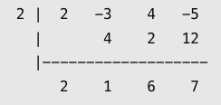
The final number is 7.

Therefore:

P(2) = 7

The final number in synthetic division is both:

• The remainder when dividing by x − 2.

• The value of the polynomial at x = 2.

This connection is one of the most useful consequences of the Remainder Theorem.

Evaluating Polynomials with Missing Terms

Some polynomials do not contain every power of x.

When using synthetic division or Horner's method, missing powers must be represented by zero coefficients.

Worked Example

Evaluate:

P(x) = x⁴ − 3x² + 5

at x = 2.

Rewrite:

P(x) = x⁴ + 0x³ − 3x² + 0x + 5

Coefficients:

1, 0, −3, 0, 5

Use synthetic division:

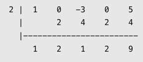
Therefore:

P(2) = 9

Check by direct substitution:

P(2) = 2⁴ − 3(2²) + 5

= 16 − 12 + 5

= 9

Both methods agree.

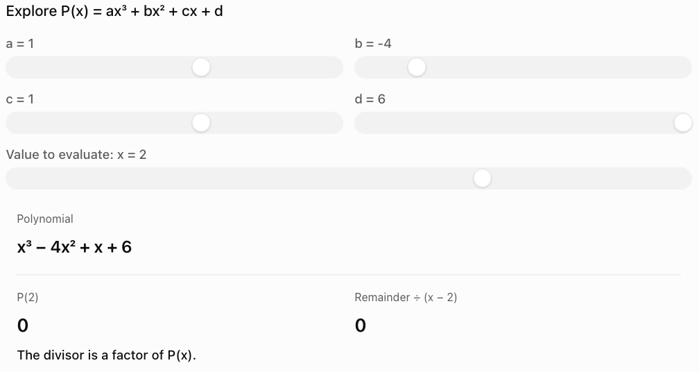
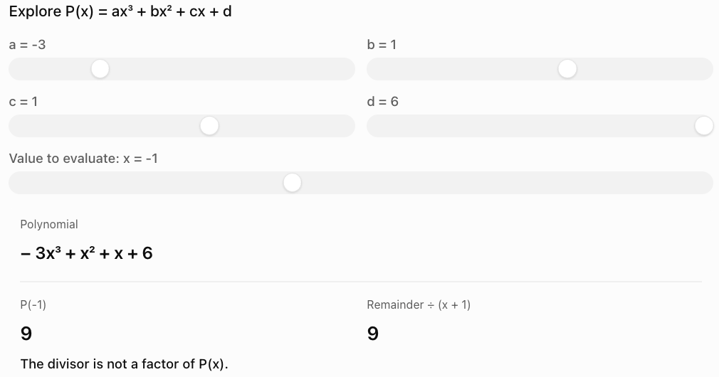
Interactive Polynomial Evaluation

Use the controls below to explore how polynomial values and remainders are connected.

The Factor Theorem

The Factor Theorem is closely related to the Remainder Theorem.

It states:

x − a is a factor of P(x) if and only if P(a) = 0.

This means that when a polynomial evaluates to zero at x = a, the expression x − a divides the polynomial exactly.

Two Important Conclusions

If:

P(a) = 0

then:

x − a is a factor of P(x).

If:

P(a) ≠ 0

then:

x − a is not a factor of P(x).

This allows us to test possible factors without performing polynomial division.

Applying the Factor Theorem

Worked Example

Determine whether:

x − 3

is a factor of:

P(x) = x² − 5x + 6

Step 1: Identify a

The divisor is x − 3.

Therefore:

a = 3

Step 2: Evaluate

P(3) = 3² − 5(3) + 6

= 9 − 15 + 6

= 0

Step 3: Interpret

Because P(3) = 0:

x − 3 is a factor of P(x).

Verification

Factor the polynomial:

x² − 5x + 6 = (x − 2)(x − 3)

The factor x − 3 appears in the product.

Testing a Binomial That Is Not a Factor

Worked Example

Determine whether:

x + 2

is a factor of:

P(x) = x³ + 2x² − 3x + 5

Step 1

The divisor is x + 2.

Therefore:

a = −2

Step 2

Evaluate:

P(−2) = (−2)³ + 2(−2)² − 3(−2) + 5

= −8 + 8 + 6 + 5

= 11

Step 3

Because:

P(−2) = 11 ≠ 0

x + 2 is not a factor of P(x).

The remainder when dividing by x + 2 is 11.

Understanding the Connection Between Factors and Zeros

Consider:

P(x) = (x − 2)(x + 3)

If x = 2:

P(2) = (2 − 2)(2 + 3)

= 0 × 5

= 0

If x = −3:

P(−3) = (−3 − 2)(−3 + 3)

= −5 × 0

= 0

Therefore, the polynomial has zeros at:

x = 2 and x = −3

The factors correspond directly to the zeros.

This is why the Factor Theorem is useful for solving polynomial equations.

The Factor Theorem and Polynomial Graphs

A zero of a polynomial is an x-value where the function equals zero.

On a graph, these values correspond to x-intercepts.

Consider:

P(x) = x² − x − 6

Factor:

P(x) = (x − 3)(x + 2)

The zeros are:

x = 3

x = −2

Therefore, the graph crosses the x-axis at:

(3, 0) and (−2, 0)

Important Connection

If P(a) = 0, then:

• a is a zero of the polynomial.

• x − a is a factor.

• (a, 0) is an x-intercept of the graph.

These are three different ways of describing the same algebraic relationship.

Using the Factor Theorem to Factor Cubic Polynomials

The Factor Theorem becomes especially useful for polynomials of degree 3 or higher.

Worked Example

Factor completely:

P(x) = x³ − 6x² + 11x − 6

Step 1: Test a Possible Zero

Try x = 1:

P(1) = 1 − 6 + 11 − 6

= 0

Therefore:

x − 1 is a factor.

Step 2: Use Synthetic Division

Divide by x − 1.

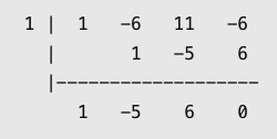
The quotient is:

x² − 5x + 6

Step 3: Factor the Quadratic

x² − 5x + 6 = (x − 2)(x − 3)

Final Answer

P(x) = (x − 1)(x − 2)(x − 3)

The zeros are:

x = 1, 2, and 3

Finding Possible Rational Zeros

When a polynomial has integer coefficients, the Rational Root Theorem can help identify possible rational zeros.

For a polynomial:

P(x) = aₙxⁿ + ... + a₁x + a₀

any rational zero p/q in lowest terms must satisfy:

• p is a factor of the constant term a₀.

• q is a factor of the leading coefficient aₙ.

Example

Consider:

P(x) = 2x³ − 3x² − 8x + 12

The constant term is 12.

The leading coefficient is 2.

Possible rational zeros include:

±1/2, ±1, ±3/2, ±2, ±3, ±4, ±6, ±12

This list contains candidates, not guaranteed zeros.

Test x = 2

P(2) = 2(8) − 3(4) − 8(2) + 12

= 16 − 12 − 16 + 12

= 0

Therefore:

x − 2 is a factor.

Synthetic Division

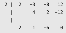
The quotient is:

2x² + x − 6

Factor:

2x² + x − 6 = (2x − 3)(x + 2)

Therefore:

P(x) = (x − 2)(2x − 3)(x + 2)

The zeros are:

x = 2, 3/2, and −2

Finding Unknown Coefficients Using the Remainder Theorem

The Remainder Theorem can help determine unknown coefficients in polynomial expressions.

Worked Example

A polynomial is defined by:

P(x) = x³ + kx² − 4x + 6

When divided by x − 2, the remainder is 10.

Find k.

Step 1: Apply the Remainder Theorem

Because the divisor is x − 2:

P(2) = 10

Step 2: Substitute

2³ + k(2²) − 4(2) + 6 = 10

Simplify:

8 + 4k − 8 + 6 = 10

4k + 6 = 10

Step 3: Solve

4k = 4

k = 1

Verification

Substitute k = 1:

P(x) = x³ + x² − 4x + 6

Evaluate:

P(2) = 8 + 4 − 8 + 6

= 10

Correct.

Finding Unknown Coefficients Using the Factor Theorem

Worked Example

Find k if x + 3 is a factor of:

P(x) = x³ + kx² − 5x + 3

Step 1: Apply the Factor Theorem

Because x + 3 is a factor:

P(−3) = 0

Step 2: Substitute

(−3)³ + k(−3)² − 5(−3) + 3 = 0

Simplify:

−27 + 9k + 15 + 3 = 0

9k − 9 = 0

Step 3: Solve

9k = 9

k = 1

Verification

P(x) = x³ + x² − 5x + 3

P(−3) = −27 + 9 + 15 + 3

= 0

Therefore, x + 3 is a factor.

Finding Two Unknown Coefficients

Sometimes a polynomial contains two unknown coefficients.

If two factors are known, we can form two equations and solve them simultaneously.

Worked Example

Suppose:

P(x) = x³ + ax² + bx + 6

Both x − 1 and x + 2 are factors.

Find a and b.

Step 1: Apply the Factor Theorem

Because x − 1 is a factor:

P(1) = 0

Because x + 2 is a factor:

P(−2) = 0

Step 2: Substitute x = 1

1 + a + b + 6 = 0

Therefore:

a + b = −7

Step 3: Substitute x = −2

−8 + 4a − 2b + 6 = 0

Simplify:

4a − 2b = 2

Divide by 2:

2a − b = 1

Step 4: Solve Simultaneously

We have:

a + b = −7

2a − b = 1

Add the equations:

3a = −6

Therefore:

a = −2

Substitute into the first equation:

−2 + b = −7

b = −5

Final Answer

a = −2 and b = −5

The polynomial is:

P(x) = x³ − 2x² − 5x + 6

Verification

P(1) = 1 − 2 − 5 + 6 = 0

P(−2) = −8 − 8 + 10 + 6 = 0

Both factors are confirmed.

Applying the Theorems to Non-Monic Linear Divisors

The standard Remainder Theorem is often stated for x − a.

However, it can also be applied to a divisor of the form:

mx + n

where m ≠ 0.

Set the divisor equal to zero:

mx + n = 0

x = −n/m

The remainder is:

R = P(−n/m)

Worked Example

Find the remainder when:

P(x) = 2x² + 3x + 5

is divided by:

2x − 1

Set the divisor equal to zero:

2x − 1 = 0

x = 1/2

Evaluate:

P(1/2) = 2(1/2)² + 3(1/2) + 5

= 2(1/4) + 3/2 + 5

= 1/2 + 3/2 + 5

= 7

Therefore:

The remainder is 7.

Generalised Factor Theorem

For m ≠ 0:

mx + n is a factor of P(x) if and only if P(−n/m) = 0.

Recognising Repeated Factors

The Factor Theorem identifies zeros, but a zero may occur more than once.

Consider:

P(x) = (x − 2)²(x + 1)

The zeros are:

x = 2

x = −1

However, x = 2 is a repeated zero because the factor x − 2 appears twice.

We say that x = 2 has multiplicity 2.

Graphical Interpretation

For a polynomial with real coefficients:

• A zero of odd multiplicity generally corresponds to the graph crossing the x-axis.

• A zero of even multiplicity generally corresponds to the graph touching the x-axis and turning around.

Worked Example

Factor:

P(x) = x³ − 3x² + 4

Test x = 2:

P(2) = 8 − 12 + 4 = 0

Therefore, x − 2 is a factor.

Synthetic division gives:

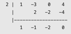
The quotient is:

x² − x − 2

Factor:

x² − x − 2 = (x − 2)(x + 1)

Therefore:

P(x) = (x − 2)²(x + 1)

The zeros are:

x = 2, with multiplicity 2.

x = −1, with multiplicity 1.

Real-World Application: Projectile Motion

Suppose the height of an object above the ground is modelled by:

h(t) = −5t² + 20t

where t is time in seconds and h is height in metres.

We want to determine when the object reaches the ground.

At ground level:

h(t) = 0

Factor:

−5t² + 20t = −5t(t − 4)

Therefore:

−5t(t − 4) = 0

Using the zero product property:

t = 0

or:

t = 4

Interpretation

At t = 0, the object is launched.

At t = 4 seconds, it returns to the ground.

The flight lasts 4 seconds.

The Factor Theorem confirms that t and t − 4 are factors of the height polynomial because h(0) = 0 and h(4) = 0.

Real-World Application: Designing a Container

Suppose the volume of a rectangular container is:

V(x) = x³ + 6x² + 11x + 6

A designer suspects that x + 1 represents one dimension.

We can test this using the Factor Theorem.

Step 1: Test the Factor

If x + 1 is a factor:

V(−1) should equal zero.

Evaluate:

V(−1) = (−1)³ + 6(−1)² + 11(−1) + 6

= −1 + 6 − 11 + 6

= 0

Therefore:

x + 1 is a factor.

Step 2: Divide

Using synthetic division with −1:

The quotient is:

x² + 5x + 6

Step 3: Factor the Quotient

x² + 5x + 6 = (x + 2)(x + 3)

Therefore:

V(x) = (x + 1)(x + 2)(x + 3)

Possible container dimensions are:

x + 1

x + 2

x + 3

For a physical container, choose x so that all three dimensions are positive.

Common Mistakes

Using the wrong substitution value

Incorrect:

For x + 4, substitute x = 4.

Correct:

For x + 4, substitute x = −4.

Confusing a nonzero remainder with a factor

If P(a) ≠ 0, then x − a is not a factor.

Forgetting missing coefficients in synthetic division

For:

x³ + 5x − 2

use coefficients:

1, 0, 5, −2

Making sign errors with negative inputs

Always use parentheses when evaluating negative values.

For example:

(−3)² = 9

Assuming a zero remainder identifies every factor

Finding one factor does not necessarily completely factor the polynomial.

Confusing zeros and factors

If x = 5 is a zero, then x − 5 is a factor.

The factor is not x + 5.

Assuming all zeros are integers

Some polynomial zeros are fractions, irrational numbers, or complex numbers.

Failing to verify unknown coefficients

After solving for an unknown coefficient, substitute it back into the original polynomial.

Using the Remainder Theorem directly with quadratic divisors

The simple evaluation rule P(a) applies to linear divisors. A quadratic divisor generally produces a remainder of degree at most 1, requiring a different approach.

Key Terms

• Polynomial: Algebraic expression containing terms with nonnegative integer exponents.

• Polynomial Function: Function defined by a polynomial expression.

• Dividend: Polynomial being divided.

• Divisor: Polynomial used to divide another polynomial.

• Quotient: Resulting polynomial in the division algorithm.

• Remainder: Expression left after polynomial division.

• Remainder Theorem: The remainder when P(x) is divided by x − a equals P(a).

• Factor Theorem: x − a is a factor of P(x) exactly when P(a) = 0.

• Factor: Expression that divides another polynomial without a remainder.

• Zero or Root: Value of x that makes a polynomial equal zero.

• x-Intercept: Point where a function's graph meets the x-axis.

• Synthetic Division: Efficient method for dividing by suitable linear expressions.

• Horner's Method: Efficient procedure for evaluating polynomials using nested multiplication.

• Coefficient: Numerical multiplier of a variable term.

• Leading Coefficient: Coefficient of the highest-degree term.

• Rational Root Theorem: Theorem that identifies possible rational zeros of polynomials with integer coefficients.

• Multiplicity: Number of times a factor occurs in the factored form of a polynomial.

• Exact Division: Division producing a zero remainder.

• Substitution: Replacing a variable with a value.

• Verification: Checking that a result satisfies the original expression or condition.

Key Takeaways

• The Remainder Theorem states that dividing P(x) by x − a gives remainder P(a).

• The Factor Theorem states that x − a is a factor exactly when P(a) = 0.

• To test x + a, substitute x = −a.

• Polynomial evaluation can replace lengthy division when only the remainder is needed.

• Horner's method provides an efficient way to evaluate polynomials.

• Synthetic division calculates both the quotient and the remainder.

• A zero remainder confirms that the divisor is a factor.

• Factors correspond to zeros of polynomial functions.

• Zeros correspond to x-intercepts on polynomial graphs.

• The Factor Theorem can help factor cubic and higher-degree polynomials.

• The Rational Root Theorem provides candidates for rational zeros.

• Unknown coefficients can be determined using given remainders or factors.

• Repeated factors correspond to zeros with multiplicity greater than one.

• These theorems are useful in algebra, geometry, physics, and mathematical modelling.

Check Your Understanding

Remainder Theorem

Find the remainder without using long division.

1. P(x) = x² + 5x + 7, divided by x − 2.

2. P(x) = x³ − 3x + 4, divided by x + 1.

3. P(x) = 2x³ + x² − 5x + 6, divided by x − 3.

4. P(x) = x⁴ − 4x² + 2, divided by x + 2.

Factor Theorem

Determine whether the given binomial is a factor.

5. P(x) = x² − 7x + 12; x − 3.

6. P(x) = x³ + 2x² − 5x − 6; x + 1.

7. P(x) = 2x³ − 3x² − 8x + 12; x − 2.

8. P(x) = x³ − 4x + 5; x + 2.

Polynomial Evaluation

9. Evaluate P(3) if P(x) = 2x³ − x² + 4x − 7.

10. Evaluate P(−2) if P(x) = x⁴ − 3x² + 2x + 1.

11. Use Horner's method to evaluate P(2) for P(x) = x³ − 5x² + 6x − 4.

12. Explain why synthetic division can be used to evaluate a polynomial.

Unknown Coefficients

13. Find k if the remainder when x² + kx + 5 is divided by x − 2 is 11.

14. Find k if x + 1 is a factor of x³ + kx² − 4x + 2.

15. Find k if x − 3 is a factor of 2x³ + kx² − 5x + 6.

Applications

16. Factor x³ − 6x² + 11x − 6 using the Factor Theorem.

17. Find the zeros of x² − 5x + 6.

18. Explain the connection between a zero, a factor, and an x-intercept.

19. Determine the remainder when P(x) = 2x² + 3x + 5 is divided by 2x − 1.

20. Explain how the Remainder and Factor Theorems are related.

Answer Key

Extended Challenge

Remainder Calculations

1. Find the remainder when 3x³ − 5x² + 7x − 4 is divided by x − 2.

2. Find the remainder when x⁴ − 2x³ + 5x − 8 is divided by x + 3.

3. Find the remainder when 2x⁵ − 3x³ + x − 7 is divided by x − 1.

4. Find the remainder when 4x³ + 2x² − 5x + 9 is divided by 2x + 1.

5. Explain how the Remainder Theorem follows from the polynomial division algorithm.

Testing Factors

6. Determine whether x − 4 is a factor of x³ − 6x² + 8x.

7. Determine whether x + 2 is a factor of 2x³ + 5x² − 4x − 12.

8. Determine whether 3x − 2 is a factor of 9x³ − 6x² − 4x + 8.

9. Find all integer zeros of x³ − 2x² − 5x + 6.

10. Factor x³ + 2x² − 9x − 18 completely.

Unknown Coefficients

11. Find k if x − 2 is a factor of x³ + kx² − 5x + 6.

12. Find k if the remainder when 2x³ + kx² − 3x + 4 is divided by x + 1 is 7.

13. Find a and b if x − 1 and x + 3 are factors of x³ + ax² + bx + 9.

14. Find a and b if P(2) = 0 and P(−1) = 0 for P(x) = 2x³ + ax² + bx − 4.

15. Construct a cubic polynomial that has zeros at x = −2, 1, and 4.

Advanced Applications

16. Use synthetic division to factor x³ − 7x + 6 completely.

17. Determine all rational zeros of 2x³ − 5x² − 4x + 3.

18. Explain why a polynomial with a repeated factor may touch the x-axis rather than cross it.

19. Show that the remainder when P(x) is divided by ax + b is P(−b/a), where a ≠ 0.

20. Construct a polynomial P(x) for which P(2) = 5 and P(−1) = −4.

Final Challenge: Polynomial Investigation

Consider the polynomial:

P(x) = x³ − 4x² − x + 4

Complete the investigation.

1. Identify the degree and leading coefficient.

2. Calculate P(1).

3. Determine whether x − 1 is a factor.

4. Calculate P(−1).

5. Determine whether x + 1 is a factor.

6. Calculate P(4).

7. Determine whether x − 4 is a factor.

8. Use synthetic division to divide P(x) by x − 1.

9. Write the resulting quotient.

10. Factor the quotient completely.

11. Write P(x) in completely factored form.

12. Identify all zeros.

13. Determine the x-intercepts of the graph.

14. Sketch the general shape of the polynomial.

15. Explain how the degree affects its end behaviour.

16. Verify the factorization by expansion.

17. Use the Remainder Theorem to calculate the remainder when dividing by x − 2.

18. Check the remainder using synthetic division.

19. Explain why x − 2 is or is not a factor.

20. Describe how the Remainder Theorem, Factor Theorem, and synthetic division work together.

Further Investigation: Creating a Polynomial with Known Remainders

Construct a polynomial of degree 3:

P(x) = ax³ + bx² + cx + d

Choose values for its coefficients so that:

• P(1) = 0

• P(−2) = 0

• P(3) = 12

Then:

1. Verify each condition using direct substitution.

2. Identify two factors of the polynomial.

3. Use synthetic division to find the remaining factor.

4. Write the polynomial in factored form.

5. Expand the factors to verify your result.

6. Explain why the polynomial is not uniquely determined by only these three conditions.

7. Investigate what additional condition would determine a unique cubic polynomial.