Analyzing and Interpreting Graphs
4. Function Features
Learning outcomes
- I can identify symmetry.
- I can identify intervals of positive and negative values.
- I can describe end behavior.
- I can compare important graph features.
- I can summarize the behavior of a graph.
Introduction
A graph provides much more information than simply showing how two variables are related. By examining its shape, position, intercepts, turning points, and overall direction, we can understand the behaviour of a function without calculating every possible output.
For example, consider the quadratic function:
f(x) = x² − 4
From its graph, we can determine that:
-
It is symmetric about the y-axis.
-
It has x-intercepts at (−2, 0) and (2, 0).
-
It has a minimum value of −4 at x = 0.
-
It is positive when x < −2 or x > 2.
-
It is negative when −2 < x < 2.
-
Both ends of the graph rise toward positive infinity.
These characteristics are called function features.
Understanding function features allows us to describe, compare, and interpret mathematical relationships in a systematic way.
This is useful in many areas of mathematics, including algebra, calculus, statistics, and mathematical modelling.
It is also important in science, engineering, economics, and other subjects where graphs are used to represent changing quantities.
What Are Function Features?
Function features are the important mathematical characteristics that describe a function's graph and behaviour.
Common features include:
-
Domain and range.
-
x-intercepts and y-intercepts.
-
Symmetry.
-
Increasing and decreasing intervals.
-
Maximum and minimum values.
-
Positive and negative intervals.
-
End behaviour.
-
Turning points.
-
Asymptotes.
-
Continuity.
Different function families have different combinations of these features.
For example, a straight line may have no turning points, while a quadratic function has one turning point.
A cubic function may have two turning points, and an exponential function may approach an asymptote without crossing it.
By identifying these features, we can build a complete mathematical description of a graph.
Symmetry of Functions
A graph has symmetry when parts of it match under a reflection or rotation.
Symmetry helps us understand graph shapes and predict values without calculating every point.
Two particularly important types of symmetry are:
-
Symmetry about the y-axis.
-
Symmetry about the origin.
These are associated with even functions and odd functions.
Even Functions: Symmetry About the y-Axis
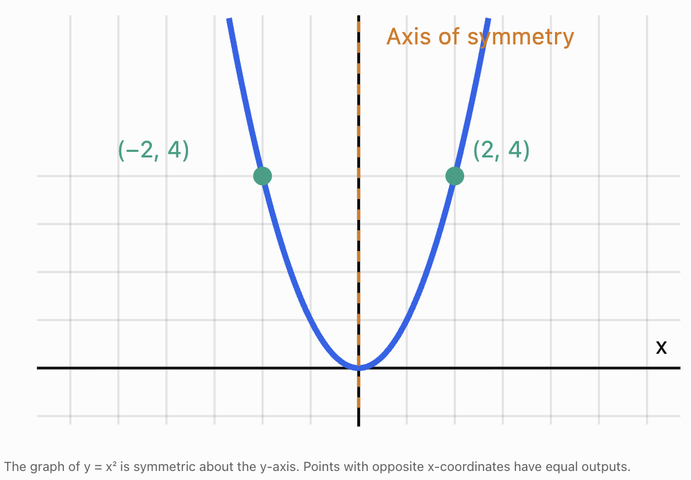
An even function has a graph that is symmetric about the y-axis.
This means the left and right sides are mirror images.
The mathematical condition is:
f(−x) = f(x)
for every x in the domain.
The domain must also be symmetric about zero.
Example: A quadratic function
Consider:
f(x) = x²
Calculate:
f(2) = 2² = 4
f(−2) = (−2)² = 4
Therefore:
f(−2) = f(2)
The same relationship holds for every real x.
The function is even.
Other examples of even functions
-
f(x) = x⁴
-
f(x) = |x|
-
f(x) = cos x
-
f(x) = x² + 5
-
f(x) = 3x⁴ − 2x² + 1
For example:
f(x) = 3x⁴ − 2x² + 1
Substitute −x:
f(−x) = 3(−x)⁴ − 2(−x)² + 1
Because even powers remove negative signs:
f(−x) = 3x⁴ − 2x² + 1
Therefore:
f(−x) = f(x)
The function is even.
Odd Functions: Symmetry About the Origin
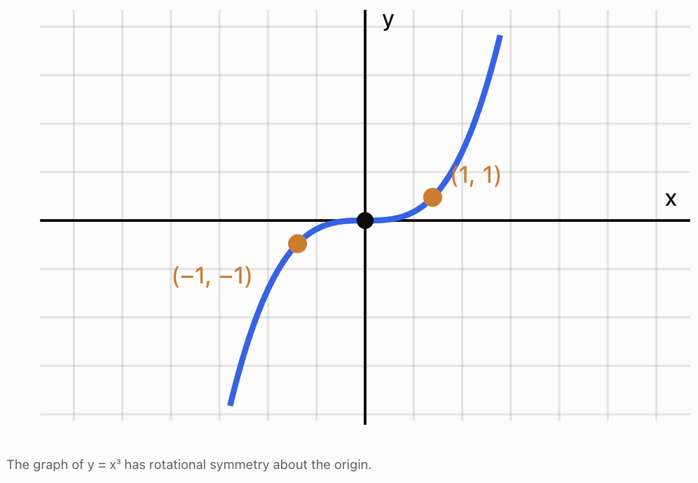
An odd function has symmetry about the origin.
This means that rotating its graph 180° around the origin produces the same graph.
The mathematical condition is:
f(−x) = −f(x)
for every x in the domain.
Example: A cubic function
Consider:
f(x) = x³
Calculate:
f(2) = 8
f(−2) = −8
Therefore:
f(−2) = −f(2)
The same relationship holds for every real x.
The function is odd.
Other examples of odd functions
-
f(x) = x
-
f(x) = x⁵
-
f(x) = sin x
-
f(x) = 1/x, for x ≠ 0
-
f(x) = x³ − 4x
Worked Example
Determine whether:
f(x) = x³ − 4x
is odd.
Substitute −x:
f(−x) = (−x)³ − 4(−x)
f(−x) = −x³ + 4x
Factor out −1:
f(−x) = −(x³ − 4x)
Therefore:
f(−x) = −f(x)
The function is odd.
Functions That Are Neither Even Nor Odd
Some functions have neither y-axis symmetry nor origin symmetry.
Consider:
f(x) = x² + x
Substitute −x:
f(−x) = x² − x
This is not equal to f(x).
It is also not equal to −f(x).
Therefore, the function is neither even nor odd.
Important distinction
A graph can have a line of symmetry without being an even function.
For example:
f(x) = (x − 3)²
has a vertical line of symmetry:
x = 3
However, it is not symmetric about the y-axis, so it is not an even function.
Similarly, some graphs have rotational symmetry around a point other than the origin without being odd functions.
Symmetry comparison
|
Feature |
Even function |
Odd function |
|---|---|---|
|
Symmetry |
y-axis |
Origin |
|
Algebraic test |
f(−x) = f(x) |
f(−x) = −f(x) |
|
Typical example |
x² |
x³ |
|
Matching points |
(x, y) and (−x, y) |
(x, y) and (−x, −y) |
The zero function f(x) = 0 is a special case: it is both even and odd.
Positive and Negative Intervals
Another important feature of a function is whether its outputs are positive or negative.
A function is positive wherever its graph lies above the x-axis.
A function is negative wherever its graph lies below the x-axis.
Mathematically:
-
Positive: f(x) > 0
-
Negative: f(x) < 0
-
Zero: f(x) = 0
These intervals describe the sign of the function's outputs, not whether the graph is increasing or decreasing.
A function can be positive and decreasing at the same time.
Worked Example: A linear function
Consider:
f(x) = 2x − 6
First, find the x-intercept:
0 = 2x − 6
x = 3
The graph crosses the x-axis at (3, 0).
For x > 3:
2x − 6 > 0
Therefore, the function is positive.
For x < 3:
2x − 6 < 0
Therefore, the function is negative.
Positive interval: (3, ∞)
Negative interval: (−∞, 3)
At x = 3, the function equals zero, so this point belongs to neither interval.
Finding Positive and Negative Intervals of Quadratic Functions
Quadratic functions can have several sign patterns depending on their roots and the direction in which they open.
Worked Example: An upward-opening parabola
Consider:
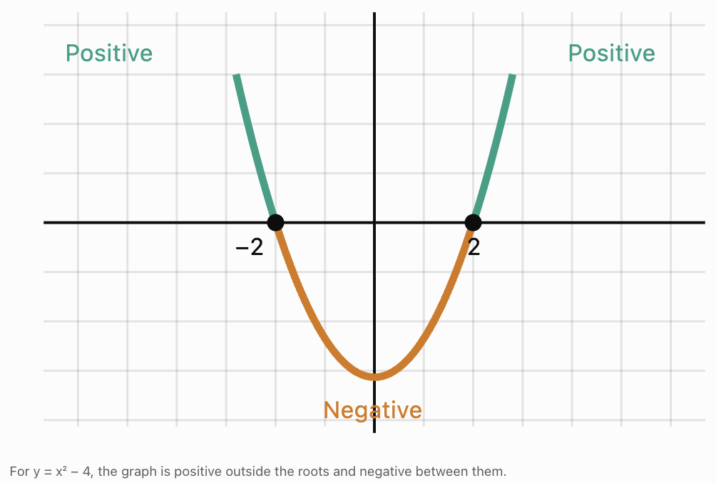
f(x) = x² − 4
Factor:
f(x) = (x − 2)(x + 2)
The roots are:
x = −2 and x = 2
These divide the number line into three intervals:
-
x < −2
-
−2 < x < 2
-
x > 2
Test one value in each interval.
|
Interval |
Test x |
f(x) |
Sign |
|---|---|---|---|
|
x < −2 |
−3 |
5 |
Positive |
|
−2 < x < 2 |
0 |
−4 |
Negative |
|
x > 2 |
3 |
5 |
Positive |
Therefore:
Positive: (−∞, −2) and (2, ∞)
Negative: (−2, 2)
Worked Example: A downward-opening parabola
Consider:
g(x) = −x² + 9
Find the roots:
0 = −x² + 9
x² = 9
x = −3 or x = 3
Since the parabola opens downward, its graph lies above the x-axis between the roots and below the x-axis outside them.
Therefore:
Positive: (−3, 3)
Negative: (−∞, −3) and (3, ∞)
A parabola that never crosses the x-axis
Consider:
h(x) = x² + 2
Since x² ≥ 0:
x² + 2 ≥ 2
Therefore, the function is positive for every real x.
Positive: (−∞, ∞)
Negative: None
This demonstrates that a function does not need x-intercepts to have positive or negative intervals.
Sign Charts
A sign chart is a useful tool for identifying where a function is positive, negative, or zero.
Consider:
f(x) = (x + 3)(x − 1)
The roots are x = −3 and x = 1.
|
Interval |
x + 3 |
x − 1 |
f(x) |
|---|---|---|---|
|
x < −3 |
Negative |
Negative |
Positive |
|
−3 < x < 1 |
Positive |
Negative |
Negative |
|
x > 1 |
Positive |
Positive |
Positive |
Multiplying two negative numbers gives a positive result.
Multiplying a positive number and a negative number gives a negative result.
Therefore:
Positive: (−∞, −3) and (1, ∞)
Negative: (−3, 1)
Sign charts are particularly useful for polynomial and rational functions.
For rational functions, remember to exclude any values where the denominator equals zero.
Distinguishing Sign from Direction of Change
One of the most important skills in graph analysis is distinguishing between the sign of a function and whether it is increasing or decreasing.
Consider:
f(x) = −x + 5
This function is decreasing everywhere because its gradient is −1.
However:
-
It is positive for x < 5.
-
It equals zero at x = 5.
-
It is negative for x > 5.
The function is therefore positive and decreasing on (−∞, 5).
Similarly, the function:
g(x) = x − 5
is increasing everywhere but negative when x < 5.
|
Feature |
Question being answered |
|---|---|
|
Positive or negative |
Is the graph above or below the x-axis? |
|
Increasing or decreasing |
Does the graph rise or fall from left to right? |
|
Maximum or minimum |
Where does the graph reach a high or low value? |
These are different properties and should be analysed separately.
End Behaviour of Functions
End behaviour describes what happens to a function's outputs as x becomes very large and positive or very large and negative.
We examine two directions:
-
As x approaches positive infinity.
-
As x approaches negative infinity.
The symbol ∞ represents infinity.
The symbol −∞ represents negative infinity.
Infinity is not a number that a function eventually reaches. Instead, these expressions describe what happens as the input grows without bound.
End behaviour notation
We commonly write:
As x → ∞, f(x) → ∞
This means that as x becomes increasingly large and positive, the output increases without bound.
Similarly:
As x → −∞, f(x) → −∞
means that as x becomes increasingly large in the negative direction, the output decreases without bound.
End behaviour helps us understand the overall shape of a graph, especially outside the visible plotting window.
End Behaviour of Linear Functions
Consider:
f(x) = 2x + 3
The gradient is positive.
Therefore:
-
As x → ∞, f(x) → ∞.
-
As x → −∞, f(x) → −∞.
Now consider:
g(x) = −2x + 3
The gradient is negative.
Therefore:
-
As x → ∞, g(x) → −∞.
-
As x → −∞, g(x) → ∞.
The sign of the gradient determines the end behaviour of a nonconstant linear function.
End Behaviour of Quadratic Functions
For:
f(x) = ax² + bx + c
the sign of a determines the end behaviour.
Positive leading coefficient
If a > 0, the parabola opens upward.
Both ends rise:
As x → ∞, f(x) → ∞
As x → −∞, f(x) → ∞
Example:
f(x) = x² − 4x + 1
Negative leading coefficient
If a < 0, the parabola opens downward.
Both ends fall:
As x → ∞, f(x) → −∞
As x → −∞, f(x) → −∞
Example:
g(x) = −2x² + 3x + 5
The lower-degree terms affect the position and shape of the graph but do not change its end behaviour.
End Behaviour of Polynomial Functions
For polynomial functions, the highest-power term usually determines the end behaviour.
This term is called the leading term.
For example:
f(x) = 3x⁴ − 2x³ + 5x − 7
The leading term is:
3x⁴
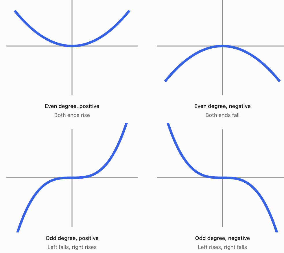
Because the degree is even and the leading coefficient is positive, both ends rise.
Four common end behaviour patterns
Summary table
|
Degree |
Leading coefficient |
Left end |
Right end |
|---|---|---|---|
|
Even |
Positive |
Rises |
Rises |
|
Even |
Negative |
Falls |
Falls |
|
Odd |
Positive |
Falls |
Rises |
|
Odd |
Negative |
Rises |
Falls |
Worked Example
Describe the end behaviour of:
f(x) = −4x⁵ + 3x² − 8
The leading term is:
−4x⁵
The degree is odd.
The leading coefficient is negative.
Therefore:
As x → −∞, f(x) → ∞
As x → ∞, f(x) → −∞
The graph rises on the left and falls on the right.
End Behaviour of Exponential Functions
Exponential functions behave differently from polynomials.
Consider:
f(x) = 2ˣ
As x becomes increasingly large:
f(x) increases without bound.
Therefore:
As x → ∞, f(x) → ∞
As x becomes increasingly negative:
f(x) approaches zero from above.
Therefore:
As x → −∞, f(x) → 0
The line y = 0 is a horizontal asymptote.
Exponential decay
Consider:
g(x) = (1/2)ˣ
As x → ∞:
g(x) → 0
As x → −∞:
g(x) → ∞
The function decreases from left to right and approaches zero on the right.
Vertical translations and asymptotes
Consider:
h(x) = 2ˣ + 3
This is the graph of 2ˣ translated upward by 3 units.
Its horizontal asymptote is:
y = 3
Therefore:
As x → −∞, h(x) → 3.
As x → ∞, h(x) → ∞.
The vertical translation changes the horizontal asymptote but does not change the overall direction of exponential growth.
End Behaviour of Rational Functions
Rational functions are ratios of polynomial expressions.
Consider:
f(x) = 1/x
As x becomes very large and positive:
f(x) approaches zero from above.
As x becomes very large and negative:
f(x) approaches zero from below.
Therefore:
-
As x → ∞, f(x) → 0.
-
As x → −∞, f(x) → 0.
The graph has a horizontal asymptote:
y = 0
It also has a vertical asymptote at:
x = 0
The function is undefined at x = 0.
Worked Example
Consider:
g(x) = 3 + 2/x
As x → ∞:
2/x → 0
Therefore:
g(x) → 3
As x → −∞:
2/x → 0
Therefore:
g(x) → 3
The horizontal asymptote is:
y = 3
This illustrates how a function can approach a finite value at both ends rather than increasing or decreasing without bound.
End Behaviour of Trigonometric Functions
Periodic functions such as sine and cosine behave differently again.
Consider:
f(x) = sin x
The function repeatedly oscillates between −1 and 1.
As x approaches positive or negative infinity, the function continues oscillating.
It does not approach one particular value.
Therefore, sin x has no single limiting value as x → ∞ or x → −∞.
This demonstrates that not all functions have end behaviour described by approaching infinity or a horizontal asymptote.
Comparing Important Graph Features
When comparing functions, it is useful to organise the information into a table.
Consider these four functions:
A: f(x) = x²
B: g(x) = −x²
C: h(x) = x³
D: p(x) = 2ˣ
Comparison table
|
Feature |
x² |
−x² |
x³ |
2ˣ |
|---|---|---|---|---|
|
Domain |
All real numbers |
All real numbers |
All real numbers |
All real numbers |
|
Range |
y ≥ 0 |
y ≤ 0 |
All real numbers |
y > 0 |
|
Symmetry |
Even |
Even |
Odd |
Neither |
|
x-intercept |
(0, 0) |
(0, 0) |
(0, 0) |
None |
|
y-intercept |
(0, 0) |
(0, 0) |
(0, 0) |
(0, 1) |
|
Extremum |
Minimum 0 |
Maximum 0 |
None |
None |
|
Positive intervals |
x ≠ 0 |
None |
x > 0 |
All real x |
|
Negative intervals |
None |
x ≠ 0 |
x < 0 |
None |
Comparing their end behaviour
f(x) = x²
Both ends rise.
g(x) = −x²
Both ends fall.
h(x) = x³
The left end falls and the right end rises.
p(x) = 2ˣ
The left end approaches zero, while the right end rises without bound.
Why comparisons matter
Although these functions may pass through some of the same points, their overall behaviour is very different.
For example, x² and x³ both pass through the origin, but:
-
x² is even.
-
x³ is odd.
-
x² has a minimum.
-
x³ has no local or absolute extrema over all real numbers.
-
x² is never negative.
-
x³ is negative for negative x-values.
Comparing several features gives a more complete understanding than looking at intercepts alone.
Summarising the Behaviour of a Graph
A complete graph description should combine several important features.
Rather than listing disconnected facts, we can explain how the function behaves as a whole.
Worked Example: A quadratic function
Consider:
f(x) = x² − 6x + 5
We will analyse its important features.
Finding the intercepts
For the x-intercepts, set f(x) = 0:
x² − 6x + 5 = 0
Factor:
(x − 1)(x − 5) = 0
Therefore:
x = 1 or x = 5
x-intercepts: (1, 0) and (5, 0)
For the y-intercept:
f(0) = 5
y-intercept: (0, 5)
Finding the turning point
Use:
x = −b/(2a)
Here a = 1 and b = −6.
x = 6/2 = 3
Substitute:
f(3) = 9 − 18 + 5
f(3) = −4
Vertex: (3, −4)
Since the parabola opens upward, this is a minimum.
Finding the symmetry
The axis of symmetry is:
x = 3
The graph is symmetric about this vertical line.
However, the function is neither even nor odd because it is not symmetric about the y-axis or origin.
Finding the positive and negative intervals
The roots are x = 1 and x = 5.
The parabola opens upward.
Therefore:
Positive: (−∞, 1) and (5, ∞)
Negative: (1, 5)
Finding increasing and decreasing intervals
The vertex occurs at x = 3.
Therefore:
Decreasing: (−∞, 3)
Increasing: (3, ∞)
Describing end behaviour
The leading term is x².
It has even degree and a positive leading coefficient.
Therefore:
-
As x → −∞, f(x) → ∞.
-
As x → ∞, f(x) → ∞.
Complete graph summary
|
Feature |
Description |
|---|---|
|
Function |
f(x) = x² − 6x + 5 |
|
Domain |
All real numbers |
|
Range |
y ≥ −4 |
|
x-intercepts |
(1, 0), (5, 0) |
|
y-intercept |
(0, 5) |
|
Minimum |
−4 at x = 3 |
|
Axis of symmetry |
x = 3 |
|
Even or odd |
Neither |
|
Increasing |
(3, ∞) |
|
Decreasing |
(−∞, 3) |
|
Positive |
(−∞, 1), (5, ∞) |
|
Negative |
(1, 5) |
|
End behaviour |
Both ends rise |
This is a complete mathematical description of the function's main features.
Real-World Application: Projectile Motion
A ball is thrown upward from a platform.
Its height is modeled by:
h(t) = −5t² + 20t + 5
where:
-
t is time in seconds.
-
h is height in metres.
Initial height
At t = 0:
h(0) = 5
The ball begins 5 m above the ground.
Maximum height
The vertex occurs at:
t = −20/[2(−5)]
t = 2
Calculate:
h(2) = −5(2)² + 20(2) + 5
h(2) = −20 + 40 + 5
h(2) = 25
Maximum height = 25 m at t = 2 s
When the ball reaches the ground
Set h(t) = 0:
−5t² + 20t + 5 = 0
Divide by −5:
t² − 4t − 1 = 0
Using the quadratic formula:
t = 2 ± √5
The positive solution is:
t ≈ 4.24 s
Interpreting the function features
Over the physical flight:
-
Height increases from t = 0 to t = 2 s.
-
Maximum height is 25 m.
-
Height decreases from t = 2 s to approximately t = 4.24 s.
-
Height is positive before the ball lands.
-
Height equals zero when the ball reaches the ground.
Although the mathematical quadratic has end behaviour extending to infinity, this is not physically meaningful for the ball's actual flight.
The practical domain is approximately:
0 ≤ t ≤ 4.24
This illustrates why real-world models must be interpreted within appropriate domains.
Real-World Application: Business Profit
Suppose a business models its profit using:
P(x) = −2(x − 30)² + 1800
where:
-
x is the number of products sold.
-
P(x) is profit in dollars.
Maximum profit
The vertex is:
(30, 1800)
Therefore:
Maximum modeled profit = $1,800
This occurs when 30 products are sold.
Positive and negative profit
A positive profit means the business earns more revenue than its costs.
A negative profit means the business operates at a loss.
Find the break-even points by setting P(x) = 0:
0 = −2(x − 30)² + 1800
2(x − 30)² = 1800
(x − 30)² = 900
x − 30 = ±30
x = 0 or x = 60
Therefore:
-
Profit is positive for 0 < x < 60.
-
Profit equals zero at x = 0 and x = 60.
-
The mathematical model gives negative profit for x > 60.
Interpreting trends
Profit increases until 30 products are sold and decreases afterward.
The function is symmetric about:
x = 30
This means equal deviations above and below 30 produce equal modeled profits.
For example:
P(20) = −2(20 − 30)² + 1800 = 1600
P(40) = −2(40 − 30)² + 1800 = 1600
Both production quantities produce a modeled profit of $1,600.
The model is illustrative and assumes the quadratic relationship remains appropriate over the quantities being considered.
Real-World Application: Population Growth
Consider:
P(t) = 500(1.08)ᵗ
where t is time in years.
The population starts at 500 and increases by 8% each year.
Function features
-
y-intercept: (0, 500).
-
Increasing for all real t mathematically.
-
Positive for all real t.
-
No x-intercept.
-
No maximum or minimum over all real t.
-
Horizontal asymptote: P = 0.
-
As t → ∞, P(t) → ∞.
-
As t → −∞, P(t) → 0.
For a real population model, we might restrict the domain to t ≥ 0.
Over this practical domain, the minimum modeled population is 500 at t = 0.
This is another example of how restricting the domain changes the extrema of a function.
A Systematic Method for Analysing Any Graph
When given a graph or equation, use the following process.
Identify the function family.
Determine whether the graph is linear, quadratic, cubic, exponential, rational, trigonometric, or another type.
Find the domain and range.
Determine the allowed input values and possible outputs.
Find the intercepts.
Calculate or estimate where the graph meets the coordinate axes.
Investigate symmetry.
Check whether the graph has y-axis symmetry, origin symmetry, or another line of symmetry.
Identify positive and negative intervals.
Find where the graph lies above and below the x-axis.
Identify increasing and decreasing intervals.
Read the graph from left to right and locate changes in direction.
Locate extrema.
Identify local and absolute maximums and minimums where they exist.
Describe end behaviour.
Explain what happens as x approaches positive and negative infinity, when this is appropriate for the domain.
Identify asymptotes or discontinuities.
Check whether the graph approaches particular lines or contains gaps.
Summarise the overall behaviour.
Combine the important features into a clear mathematical description.
Common Mistakes
Confusing symmetry about the y-axis with symmetry about another vertical line
A parabola with axis x = 3 is not necessarily an even function.
Assuming every function is even or odd
Many functions are neither.
Confusing positive intervals with increasing intervals
Positive means the output is above zero. Increasing means the output rises as x increases.
Including roots in strictly positive or negative intervals
At an x-intercept, f(x) = 0, so the function is neither positive nor negative.
Describing end behaviour using only the visible graph
A plotting window may not show the long-term behaviour of a function.
Ignoring the leading coefficient
For polynomial functions, the sign of the leading coefficient affects the direction of the graph's ends.
Assuming all functions approach infinity at their ends
Exponential and rational functions may approach finite asymptotes, while trigonometric functions may oscillate indefinitely.
Confusing an asymptote with an intercept
An asymptote describes limiting behaviour, while an intercept is a point on the graph.
Assuming symmetry guarantees a maximum or minimum
For example, y = x³ has origin symmetry but no maximum or minimum over all real numbers.
Ignoring domain restrictions
A real-world model may only apply over a limited interval, changing which features are relevant.
Key Terms
-
Function feature: A mathematical characteristic describing a graph or function.
-
Symmetry: A property in which a graph matches itself under a reflection or rotation.
-
Even function: A function satisfying f(−x) = f(x).
-
Odd function: A function satisfying f(−x) = −f(x).
-
Axis of symmetry: A line dividing a graph into mirror-image halves.
-
Origin symmetry: Symmetry under a 180° rotation about the origin.
-
Positive interval: An interval where f(x) > 0.
-
Negative interval: An interval where f(x) < 0.
-
Root or zero: An input value where f(x) = 0.
-
Sign chart: A table showing where an expression is positive or negative.
-
End behaviour: The behaviour of a function as its input approaches positive or negative infinity.
-
Leading term: The term containing the highest power in a polynomial.
-
Leading coefficient: The coefficient of the highest-power term.
-
Degree: The highest exponent of the variable in a polynomial.
-
Asymptote: A line that a graph approaches in a specified limiting direction.
-
Horizontal asymptote: A horizontal line approached by a graph as x approaches positive or negative infinity.
-
Vertical asymptote: A vertical line near which a function becomes unbounded on at least one side.
-
Increasing interval: An interval where outputs rise as inputs increase.
-
Decreasing interval: An interval where outputs fall as inputs increase.
-
Extremum: A maximum or minimum value.
-
Turning point: A point where a graph changes from increasing to decreasing or vice versa.
-
Domain: The set of allowed input values.
-
Range: The set of possible output values.
Key Takeaways
-
Function features provide a systematic way to describe and compare graphs.
-
Even functions have y-axis symmetry and satisfy f(−x) = f(x).
-
Odd functions have origin symmetry and satisfy f(−x) = −f(x).
-
A function may be neither even nor odd.
-
Positive intervals occur where the graph lies above the x-axis.
-
Negative intervals occur where the graph lies below the x-axis.
-
Positive and negative intervals are different from increasing and decreasing intervals.
-
End behaviour describes how a function behaves as x approaches positive or negative infinity.
-
The leading term determines the end behaviour of a nonconstant polynomial.
-
Exponential and rational functions may approach horizontal asymptotes.
-
Periodic functions may continue oscillating rather than approaching a single value.
-
Graphs can be compared using intercepts, symmetry, extrema, intervals, and end behaviour.
-
Real-world graph analysis must consider the practical domain and meaning of the variables.
Check Your Understanding
Recall and Understanding
1. What is an even function? State the algebraic condition used to identify one.
2. What is an odd function? Describe its graphical symmetry.
3. Explain the difference between a positive interval and an increasing interval.
4. What is meant by the end behaviour of a function?
5. Why is the leading term important when describing the end behaviour of a polynomial?
Application
6. Determine whether f(x) = 4x⁴ − 3x² + 2 is even, odd, or neither.
7. Determine whether g(x) = 2x³ − 5x is even, odd, or neither.
8. Find the positive and negative intervals of f(x) = x² − 9.
9. Find the positive and negative intervals of g(x) = −x² + 16.
10. Describe the end behaviour of f(x) = 3x⁴ − 2x + 7.
11. Describe the end behaviour of g(x) = −2x⁵ + x³ − 4.
12. Determine the horizontal asymptote and end behaviour of h(x) = 3ˣ + 2.
Analysis and Challenge
13. Analyse f(x) = x² − 4x + 3. Identify its intercepts, axis of symmetry, minimum, positive and negative intervals, increasing and decreasing intervals, and end behaviour.
14. Compare the symmetry, extrema, and end behaviour of f(x) = x² and g(x) = −x³.
15. A student claims that f(x) = (x − 2)² is even because its graph has a vertical axis of symmetry. Explain the error.
Answers to Check Your Understanding
1. An even function has symmetry about the y-axis and satisfies:
f(−x) = f(x)
for every input in its domain.
2. An odd function has symmetry about the origin. Rotating its graph 180° around the origin produces the same graph.
Its algebraic condition is:
f(−x) = −f(x)
3. A positive interval is where f(x) > 0, meaning the graph is above the x-axis. An increasing interval is where the output rises as x increases.
4. End behaviour describes what happens to the outputs as x approaches positive or negative infinity.
5. For a polynomial, the leading term dominates the lower-degree terms when the magnitude of x becomes very large. Its degree and coefficient determine the graph's end behaviour.
6.
f(x) = 4x⁴ − 3x² + 2
f(−x) = 4(−x)⁴ − 3(−x)² + 2
f(−x) = 4x⁴ − 3x² + 2
Therefore:
The function is even.
7.
g(x) = 2x³ − 5x
g(−x) = −2x³ + 5x
g(−x) = −g(x)
Therefore:
The function is odd.
8.
f(x) = x² − 9
Factor:
f(x) = (x − 3)(x + 3)
Roots:
x = −3 and x = 3
Since the parabola opens upward:
Positive: (−∞, −3) and (3, ∞)
Negative: (−3, 3)
9.
g(x) = −x² + 16
Set g(x) = 0:
x² = 16
x = −4 or x = 4
The parabola opens downward.
Positive: (−4, 4)
Negative: (−∞, −4) and (4, ∞)
10.
f(x) = 3x⁴ − 2x + 7
The leading term is 3x⁴.
It has even degree and a positive leading coefficient.
Therefore:
As x → −∞, f(x) → ∞
As x → ∞, f(x) → ∞
Both ends rise.
11.
g(x) = −2x⁵ + x³ − 4
The leading term is −2x⁵.
It has odd degree and a negative leading coefficient.
Therefore:
As x → −∞, g(x) → ∞
As x → ∞, g(x) → −∞
The left end rises and the right end falls.
12.
h(x) = 3ˣ + 2
The parent exponential function is shifted upward by 2.
Horizontal asymptote:
y = 2
End behaviour:
As x → −∞, h(x) → 2.
As x → ∞, h(x) → ∞.
13.
f(x) = x² − 4x + 3
Factor:
f(x) = (x − 1)(x − 3)
x-intercepts:
(1, 0) and (3, 0)
y-intercept:
f(0) = 3
(0, 3)
Vertex x-coordinate:
x = −(−4)/(2 × 1) = 2
Vertex y-coordinate:
f(2) = 4 − 8 + 3 = −1
Minimum point:
(2, −1)
Axis of symmetry:
x = 2
Positive intervals:
(−∞, 1) and (3, ∞)
Negative interval:
(1, 3)
Decreasing interval:
(−∞, 2)
Increasing interval:
(2, ∞)
End behaviour:
Both ends rise toward positive infinity.
The function is neither even nor odd.
14.
For f(x) = x²:
-
Even function.
-
Symmetric about the y-axis.
-
Minimum value 0 at x = 0.
-
Both ends rise toward positive infinity.
For g(x) = −x³:
-
Odd function.
-
Symmetric about the origin.
-
No local or absolute extrema over all real numbers.
-
Left end rises toward positive infinity.
-
Right end falls toward negative infinity.
Both functions pass through the origin, but their symmetry and end behaviour differ.
15.
The function:
f(x) = (x − 2)²
has a vertical axis of symmetry at:
x = 2
However, an even function must be symmetric specifically about the y-axis.
Check algebraically:
f(−x) = (−x − 2)² = (x + 2)²
This is not generally equal to (x − 2)².
Therefore:
The function is neither even nor odd.
Final Summary
Function features allow us to understand the overall behaviour of graphs by examining symmetry, positive and negative intervals, end behaviour, intercepts, extrema, and changes in direction.
By combining these characteristics, we can describe functions accurately, compare different mathematical relationships, and interpret graphs in real-world contexts.
A complete understanding of a graph comes from examining how its important features work together, rather than studying each feature separately.