Applications of Sequences and Series
4. Mathematical Modeling Project
Learning outcomes
- I can collect and organize data related to a real-world pattern.
- I can identify whether a pattern is arithmetic, geometric, or recursive.
- I can develop a mathematical model to describe a pattern.
- I can use my model to make predictions.
- I can communicate my findings using mathematical language and representations.
Introduction
Mathematics is not only about solving equations or identifying patterns in numbers. It is also a powerful tool for understanding the real world.
Scientists use mathematical models to predict population growth. Engineers use them to describe motion and mechanical systems. Economists use models to investigate financial changes, while environmental researchers use them to study resource consumption and sustainability.
In each case, the process begins with observations and data.
For example, imagine recording the distance travelled by a small robot every second:
0, 12, 24, 36, 48, 60, ...
The data suggest that the robot travels the same distance during every second. We can represent this pattern using an arithmetic sequence and develop a model that predicts future positions.
Now consider a bacterial population:
100, 150, 225, 337.5, ...
The population increases by 50% during each time interval. This suggests a geometric model.
But what happens when a pattern is more complicated? What if a population grows while resources become limited, or an investment receives additional deposits every month?
These situations may require recursive models or other mathematical relationships.
In this project, you will become a mathematical investigator. You will collect or obtain real-world data, organise the information, identify patterns, develop a mathematical model, make predictions, and communicate your findings.
The goal is not simply to find an equation. It is to explain why a particular mathematical model is appropriate, how well it represents the data, and what its predictions mean in the real world.
What Is Mathematical Modeling?
Mathematical modeling is the process of representing a real-world situation using mathematical relationships.
A mathematical model may include:
-
Equations
-
Functions
-
Sequences
-
Tables
-
Graphs
-
Recursive rules
-
Diagrams
-
Statistical relationships
-
Computer simulations
Models help us simplify complicated situations so that we can investigate important relationships.
For example, suppose a water tank contains 1,000 litres of water and loses 40 litres every hour.
A mathematical model is:
Wₙ = 1,000 − 40n
where:
-
Wₙ = water remaining after n hours
-
n = number of hours
The model predicts that after six hours:
W₆ = 1,000 − 40(6)
= 760
Predicted water remaining = 760 litres
However, the model assumes that water is lost at a constant rate.
If the rate changes, the model may become inaccurate.
This illustrates a central idea:
A mathematical model is a simplified representation of reality, not a perfect description of it.
The Mathematical Modeling Cycle
Mathematical modeling is an investigation that often involves repeating several steps.
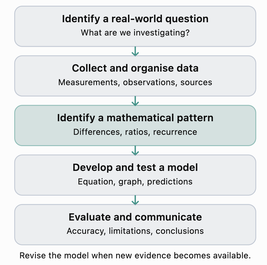
The five main stages are:
-
Define a question that can be investigated mathematically.
-
Collect and organise relevant data.
-
Identify the pattern or relationship.
-
Develop a model and use it to make predictions.
-
Evaluate the model and communicate the findings.
These stages do not always occur in a fixed order. Investigators may return to earlier stages when new evidence reveals a problem.
Choosing a Real-World Investigation
The first step is selecting a situation that produces measurable or countable data.
A suitable project should have:
-
A clearly defined quantity to investigate.
-
A measurable independent variable, often time or event number.
-
Enough data to identify a possible pattern.
-
A mathematical relationship that can be investigated.
-
Opportunities to make and test predictions.
Suggested project topics
|
Project idea |
Quantity measured |
Possible model |
|---|---|---|
|
Walking at constant speed |
Distance over time |
Arithmetic |
|
Bouncing ball |
Maximum height after each bounce |
Geometric |
|
Savings account |
Balance after each interest period |
Geometric |
|
Saving with regular deposits |
Account balance |
Recursive |
|
Water consumption |
Water remaining over time |
Arithmetic or recursive |
|
Plant growth |
Height over time |
Linear or nonlinear |
|
Population growth |
Number of organisms |
Geometric or logistic |
|
Cooling object |
Temperature difference from surroundings |
Geometric approximation |
|
Machine production |
Total items produced |
Arithmetic |
|
Repeated folding |
Number of layers |
Geometric |
|
Pendulum |
Completion time of each oscillation |
Arithmetic |
|
Resource harvesting |
Resource remaining |
Recursive |
A project should be chosen based on the available data rather than assuming in advance that a particular mathematical model will fit.
Collecting Real-World Data
Data collection is the foundation of mathematical modeling.
Poor-quality data can produce misleading conclusions, even when the calculations are correct.
Primary data
Primary data are collected directly by the investigator.
Examples include:
-
Measuring a ball's rebound heights.
-
Timing a moving object.
-
Recording plant height over several days.
-
Measuring water levels in a container.
-
Counting objects produced during repeated cycles.
Secondary data
Secondary data come from existing sources.
Examples include:
-
Published population statistics.
-
Historical financial information.
-
Weather records.
-
Environmental measurements.
-
Scientific databases.
When using secondary data, record the source and explain whether it is reliable and relevant.
Designing a data collection plan
Before collecting data, decide:
-
What quantity will be measured?
-
What units will be used?
-
How often will measurements be taken?
-
How many observations are needed?
-
What equipment or sources will be used?
-
What factors might affect the measurements?
-
How will the data be recorded?
A practical starting target is at least eight to ten observations, although some investigations may require more.
For experiments, repeated trials can help assess measurement variability.
Organising Data in Tables
A clear data table makes patterns easier to recognise.
Suppose a student measures the cumulative distance travelled by a robot every second.
|
Time (s) |
Distance (cm) |
|---|---|
|
0 |
0 |
|
1 |
14 |
|
2 |
28 |
|
3 |
42 |
|
4 |
56 |
|
5 |
70 |
|
6 |
84 |
The table shows that the distance increases by 14 cm every second.
This suggests an arithmetic sequence.
Important features of a good data table
-
Clear column headings.
-
Correct units.
-
Consistent measurement intervals when possible.
-
Values recorded with appropriate precision.
-
No unexplained missing measurements.
-
A logical ordering of observations.
For real experimental data, measurements may not follow an exact mathematical pattern.
For example:
0, 13.8, 28.1, 41.7, 56.2, 70.0, 83.9
These measurements still suggest approximately constant-speed motion.
The purpose of modeling is to identify a useful relationship, not to force every measurement into an exact sequence.
Identifying Arithmetic Patterns
An arithmetic sequence has a constant difference between consecutive terms.
The general explicit formula is:
aₙ = a₀ + nd
where:
-
a₀ = initial value
-
d = common difference
-
n = number of intervals
The recursive form is:
aₙ₊₁ = aₙ + d
Worked Example 1: Water Consumption
A water container initially holds 500 litres.
Measurements show:
|
Hour |
Water remaining (L) |
|---|---|
|
0 |
500 |
|
1 |
465 |
|
2 |
430 |
|
3 |
395 |
|
4 |
360 |
Step 1: Calculate the differences.
465 − 500 = −35
430 − 465 = −35
395 − 430 = −35
360 − 395 = −35
The common difference is −35.
Step 2: Identify the model.
The data follow an arithmetic sequence.
Step 3: Write an explicit model.
Wₙ = 500 − 35n
Step 4: Write a recursive model.
W₀ = 500
Wₙ₊₁ = Wₙ − 35
Step 5: Make a prediction.
After eight hours:
W₈ = 500 − 35(8)
= 500 − 280
W₈ = 220 litres
Evaluating the model
The model assumes water consumption remains constant.
It is useful only while water remains in the container and the consumption rate stays unchanged.
Identifying Geometric Patterns
A geometric sequence has a constant ratio between consecutive terms.
The explicit formula is:
aₙ = a₀rⁿ
where r is the common ratio.
The recursive form is:
aₙ₊₁ = raₙ
Worked Example 2: Bouncing Ball
A ball is dropped from 2 metres.
The recorded maximum heights are:
|
Bounce number |
Maximum height (m) |
|---|---|
|
0 |
2.000 |
|
1 |
1.600 |
|
2 |
1.280 |
|
3 |
1.024 |
|
4 |
0.8192 |
Step 1: Calculate the ratios.
1.600/2.000 = 0.8
1.280/1.600 = 0.8
1.024/1.280 = 0.8
0.8192/1.024 = 0.8
Step 2: Identify the model.
The sequence is geometric.
Step 3: Write the model.
hₙ = 2(0.8)ⁿ
Step 4: Predict the height after seven bounces.
h₇ = 2(0.8)⁷
= 2(0.2097152)
= 0.4194304
Predicted height ≈ 0.419 m
Evaluating the model
The model assumes that the ball rebounds to exactly 80% of its previous height.
Actual rebound ratios may vary because of surface conditions, deformation, spin, and measurement error.
Identifying Recursive Patterns
Some real-world processes depend on the previous value and an additional change.
These can be represented using recursive models.
For example, suppose an account:
-
Begins with $1,000.
-
Earns 5% interest each year.
-
Receives a $200 deposit at the end of each year.
The recursive rule is:
Aₙ₊₁ = 1.05Aₙ + 200
with:
A₀ = 1,000
Worked Example 3: Investment with Regular Deposits
Calculate the first four year-end balances.
Year 1:
A₁ = 1.05(1,000) + 200
= 1,250
Year 2:
A₂ = 1.05(1,250) + 200
= 1,512.50
Year 3:
A₃ = 1.05(1,512.50) + 200
= 1,788.125
Year 4:
A₄ = 1.05(1,788.125) + 200
= 2,077.53125
Predicted balance after four years: $2,077.53
This model is recursive because each new balance depends on the previous balance.
It is not a simple geometric sequence because the fixed deposit changes the ratio between consecutive balances.
An important distinction
Arithmetic and geometric sequences can both be described recursively.
However, not every recursive sequence is arithmetic or geometric.
A recursive model may combine addition, multiplication, subtraction, or more complicated relationships.
Comparing Mathematical Models
Choosing a mathematical model requires examining the structure of the data.
|
Feature |
Arithmetic model |
Geometric model |
General recursive model |
|---|---|---|---|
|
Main pattern |
Constant difference |
Constant ratio |
New value depends on previous value(s) |
|
Typical rule |
aₙ₊₁ = aₙ + d |
aₙ₊₁ = raₙ |
aₙ₊₁ = f(aₙ, n) |
|
Explicit formula |
aₙ = a₀ + nd |
aₙ = a₀rⁿ |
May or may not have a simple explicit formula |
|
Common application |
Constant consumption |
Repeated percentage growth |
Growth with deposits or harvesting |
|
Graph pattern |
Straight line at equally spaced times |
Exponential curve |
Depends on the rule |
A model selection strategy
First, calculate the differences between consecutive terms.
If the differences are approximately constant, consider an arithmetic model.
Next, calculate ratios between consecutive nonzero terms.
If the ratios are approximately constant, consider a geometric model.
If neither pattern fits, investigate whether the process can be described using a recursive rule.
Other possibilities include quadratic, logistic, periodic, and statistical models.
Do not assume that all real-world patterns must be arithmetic, geometric, or recursive in a particular simple form.
Investigating Patterns Using Graphs
Graphs provide a visual representation of mathematical relationships.
A graph can reveal:
-
Increasing or decreasing trends.
-
Constant rates of change.
-
Exponential growth or decay.
-
Curved relationships.
-
Unusual observations.
-
Possible limitations of a model.
Comparing two models
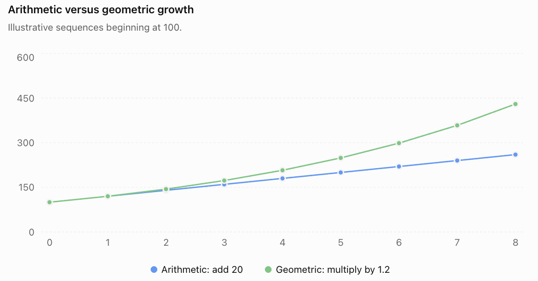
The arithmetic model increases by equal amounts.
The geometric model increases by equal percentages.
The geometric sequence eventually grows much faster.
Graphing real measurements
When graphing experimental data:
-
Place the independent variable on the horizontal axis.
-
Place the dependent variable on the vertical axis.
-
Label both axes and include units.
-
Choose a suitable scale.
-
Plot the observed values.
-
Add the mathematical model for comparison.
-
Look for systematic differences between the data and the model.
A graph should help explain the investigation rather than simply decorate the report.
Developing a Mathematical Model
After identifying a possible pattern, construct a formula.
Step 1: Define the variables
For example:
n = number of days
Pₙ = population after n days
Step 2: Identify the initial value
Suppose:
P₀ = 200
Step 3: Determine the pattern
If the population increases by 15% each day:
Growth factor = 1.15
Step 4: Write the model
Pₙ = 200(1.15)ⁿ
Step 5: Test the model
After one day:
P₁ = 200(1.15) = 230
After two days:
P₂ = 200(1.15)² = 264.5
Compare these predictions with the observed data.
Step 6: Interpret the model
The model assumes that the population increases by 15% every day.
It may be appropriate for a short period but unrealistic over a long period because resources are limited.
Testing Model Accuracy
A mathematical model should be evaluated using the available data.
One simple method is to calculate the difference between observed and predicted values.
This difference is called a residual.
Residual = Observed value − Predicted value
Worked Example 4: Testing a Motion Model
A student proposes the model:
d = 5t
where d is distance in metres and t is time in seconds.
The observed measurements are:
|
Time (s) |
Observed distance (m) |
Predicted distance (m) |
Residual (m) |
|---|---|---|---|
|
1 |
5.2 |
5 |
+0.2 |
|
2 |
9.8 |
10 |
−0.2 |
|
3 |
15.3 |
15 |
+0.3 |
|
4 |
19.7 |
20 |
−0.3 |
|
5 |
25.1 |
25 |
+0.1 |
The residuals are small compared with the measured distances.
This suggests that the model provides a reasonable approximation for these observations.
However, model accuracy should not be judged only by whether residuals are small. We should also check whether residuals show a pattern and whether the model makes physical sense.
Mean absolute error
One simple measure of overall prediction error is the mean absolute error (MAE).
MAE = Sum of absolute residuals ÷ Number of observations
For this example:
MAE = (0.2 + 0.2 + 0.3 + 0.3 + 0.1)/5
= 1.1/5
MAE = 0.22 m
A smaller MAE indicates smaller average absolute prediction errors, although comparisons are most meaningful when models are evaluated on comparable data and units.
Making Predictions
One of the main purposes of a mathematical model is to predict future values.
There are two important types of prediction.
Interpolation
Interpolation estimates a value within the range of observed data.
For example, if a robot's position is measured at 2 seconds and 4 seconds, a model may estimate its position at 3 seconds.
Extrapolation
Extrapolation predicts values outside the observed data range.
For example, using measurements from the first five seconds to predict the robot's position after twenty seconds is extrapolation.
Extrapolation is generally more uncertain because the pattern may change beyond the observed period.
Worked Example 5: Predicting Population Growth
A population begins with 500 organisms and grows by 8% each year.
Predict the population after ten years.
Use:
Pₙ = 500(1.08)ⁿ
P₁₀ = 500(1.08)¹⁰
≈ 500(2.158925)
≈ 1,079.46
Predicted population: approximately 1,079 organisms
This prediction assumes the 8% growth rate remains constant.
Evaluating the Limitations of a Model
A model may fit existing data but still produce unreliable future predictions.
Important questions include:
1. Are the assumptions realistic?
A model may assume constant speed, constant growth, or constant consumption.
2. Is the data reliable?
Measurements may contain errors or inconsistencies.
3. Is the model appropriate for the time period?
A short-term model may not remain valid over many years.
4. Are important variables missing?
Population models may ignore resources, disease, or migration.
5. Does the model respect physical constraints?
A water model should not predict negative water quantities as physically meaningful.
6. How accurately does the model fit the data?
Residuals and graphs can reveal poor fits.
7. How uncertain are the predictions?
Future outcomes may differ if conditions change.
8. Could another model provide a better explanation?
Different models may fit the same limited dataset but produce different long-term predictions.
A strong mathematical investigation discusses limitations rather than pretending that the model is perfect.
Communicating Mathematical Findings
Mathematical communication involves explaining the investigation clearly enough that another person can understand and evaluate it.
A good report should include:
-
A clearly stated research question.
-
An explanation of the real-world situation.
-
A description of how data were collected.
-
A table of observations.
-
A graph showing the data.
-
Identification of the mathematical pattern.
-
A mathematical model with defined variables.
-
Worked calculations.
-
Predictions based on the model.
-
Evaluation of model accuracy.
-
Discussion of assumptions and limitations.
-
A conclusion supported by evidence.
Mathematical vocabulary
Use precise mathematical language.
Instead of writing:
"The numbers keep getting bigger."
Write:
"The data show an approximately constant positive difference, suggesting an arithmetic sequence."
Instead of writing:
"The amount gets smaller every time."
Write:
"The values decrease by approximately 15% during each interval, suggesting geometric decay with a common ratio of 0.85."
Instead of writing:
"The model works."
Write:
"The model provides a reasonable approximation over the observed interval, although its predictions may become less reliable beyond the measured data."
Clear mathematical communication explains both the calculations and their meaning.
Mathematical Modeling Project: Student Investigation
Project Overview
You will investigate a real-world pattern and develop a mathematical model that explains the relationship between two quantities.
Your project must include original measurements or a clearly identified dataset, mathematical analysis, a model, predictions, and an evaluation.
Project goal
Develop and evaluate a mathematical model that describes a real-world pattern using arithmetic, geometric, or recursive relationships.
Suggested time
Approximately 4–6 lessons, plus any additional time needed for data collection.
Project requirements
Your investigation must include all of the following:
-
A research question.
-
A description of the situation.
-
At least eight observations, where practical.
-
A clearly organised data table.
-
A graph of the observations.
-
Analysis of differences, ratios, or recursive relationships.
-
A mathematical model.
-
At least two predictions.
-
A comparison between predictions and observations where possible.
-
A discussion of assumptions, limitations, and possible improvements.
-
A final conclusion using appropriate mathematical language.
Stage 1: Planning the Investigation
Begin by choosing a real-world situation.
Possible examples include:
-
How does a bouncing ball's height change after each bounce?
-
How does the distance travelled by a robot change over time?
-
How does a savings balance grow with repeated deposits?
-
How does water remaining in a container change during constant consumption?
-
How does a plant's height change over several days?
-
How does a rotating wheel's cumulative number of revolutions change over time?
Planning organiser
Project title: __________________________
Research question: __________________________
Independent variable: __________________________
Dependent variable: __________________________
Units of measurement: __________________________
Data collection method: __________________________
Number of observations planned: __________________________
Possible mathematical pattern: __________________________
Factors that may affect the data: __________________________
Stage 2: Collecting and Organising Data
Record your observations in a table.
|
Observation number |
Independent variable |
Measured value |
Notes |
|---|---|---|---|
|
1 |
|||
|
2 |
|||
|
3 |
|||
|
4 |
|||
|
5 |
|||
|
6 |
|||
|
7 |
|||
|
8 |
|||
|
9 |
|||
|
10 |
Include units in the column headings when completing the table.
If you conduct repeated trials, record each trial and calculate appropriate summary values.
Stage 3: Identifying the Pattern
Calculate the differences between consecutive values.
Difference = Current value − Previous value
If the values are nonzero, calculate the ratios.
Ratio = Current value ÷ Previous value
Use these calculations to investigate whether the data are approximately arithmetic or geometric.
If neither pattern is appropriate, investigate a recursive relationship or another mathematical model.
Pattern analysis questions
-
Does the quantity increase, decrease, or remain constant?
-
Are the first differences approximately constant?
-
Are the ratios approximately constant?
-
Does the pattern appear linear, exponential, or more complicated?
-
Is there a physical reason why the pattern might occur?
-
Which mathematical model seems most appropriate?
Stage 4: Developing the Model
Write an equation or recursive rule describing the pattern.
For an arithmetic model:
aₙ = a₀ + nd
For a geometric model:
aₙ = a₀rⁿ
For a recursive model:
aₙ₊₁ = f(aₙ, n)
Explain:
-
What each variable represents.
-
How the parameters were determined.
-
Why the model was selected.
-
Whether the model fits the observed data.
If the measurements are not exact, explain how you estimated the parameters.
Stage 5: Making Predictions
Use the model to calculate at least two values that were not used to construct it.
For example:
-
Predict the next observation.
-
Predict a value several periods into the future.
-
Estimate when a quantity will reach a target.
-
Determine when a resource may be exhausted.
-
Estimate how many cycles are needed for a quantity to halve.
Show the calculations and include units.
Whenever possible, collect additional data to test one of your predictions.
Stage 6: Evaluating the Model
Write an evaluation addressing:
-
How accurately does the model represent the observations?
-
Which observations differ most from the predictions?
-
What assumptions were necessary?
-
What measurement errors may have occurred?
-
What real-world factors were excluded?
-
How reliable are predictions beyond the observed data?
-
What could be improved in a future investigation?
An effective evaluation uses specific evidence from the investigation.
Stage 7: Presenting the Findings
Prepare a mathematical investigation report or presentation.
Suggested report structure
Title
A clear description of the investigation.
Introduction
Explain the real-world situation and research question.
Methodology
Describe how the data were collected or obtained.
Data and Results
Present tables and graphs.
Mathematical Analysis
Identify the pattern and explain the mathematical model.
Predictions
Show calculations and interpret predicted values.
Evaluation
Discuss model accuracy, assumptions, and limitations.
Conclusion
Summarise the findings and explain what the mathematical model reveals.
References
Identify any external datasets, sources, or supporting information.
Project Assessment Rubric
Suggested assessment: 40 marks
|
Criterion |
Marks |
Expectations |
|---|---|---|
|
Research question and planning |
5 |
Clear question, appropriate variables, suitable data collection plan |
|
Data collection and organisation |
7 |
Sufficient relevant data, accurate measurements, clear tables and units |
|
Pattern identification |
6 |
Correct differences, ratios, and mathematical classification |
|
Mathematical model |
8 |
Appropriate model, correctly defined variables, accurate calculations |
|
Predictions and interpretation |
6 |
Meaningful predictions, correct calculations, interpretation in context |
|
Evaluation and communication |
8 |
Thoughtful limitations, clear graphs, precise terminology, organised conclusions |
|
Total |
40 |
What distinguishes an excellent project?
An excellent investigation does more than produce a correct equation.
It demonstrates that the student understands the relationship between the real-world situation and the mathematics.
The model is justified using evidence, predictions are interpreted meaningfully, and limitations are evaluated carefully.
Fully Worked Sample Project
Investigating the Height of a Bouncing Ball
Research question: How does the maximum rebound height of a ball change after successive bounces?
Hypothesis
The ball will rebound to approximately the same fraction of its previous maximum height after each bounce.
Therefore, the rebound heights may follow a geometric sequence.
Data
The following is an illustrative dataset rather than measurements from a real experiment.
|
Bounce number |
Maximum height (cm) |
|---|---|
|
0 |
200 |
|
1 |
160 |
|
2 |
128 |
|
3 |
102 |
|
4 |
82 |
|
5 |
66 |
Pattern analysis
Calculate the ratios:
160/200 = 0.800
128/160 = 0.800
102/128 ≈ 0.797
82/102 ≈ 0.804
66/82 ≈ 0.805
The ratios are approximately constant.
The common ratio is close to 0.80.
This suggests a geometric model.
Mathematical model
Initial height:
h₀ = 200 cm
Estimated common ratio:
r = 0.80
Explicit model:
hₙ = 200(0.80)ⁿ
Recursive model:
hₙ₊₁ = 0.80hₙ
Testing the model
|
Bounce |
Observed height (cm) |
Predicted height (cm) |
Residual (cm) |
|---|---|---|---|
|
0 |
200 |
200.00 |
0.00 |
|
1 |
160 |
160.00 |
0.00 |
|
2 |
128 |
128.00 |
0.00 |
|
3 |
102 |
102.40 |
−0.40 |
|
4 |
82 |
81.92 |
+0.08 |
|
5 |
66 |
65.54 |
+0.46 |
The predictions are close to the observed values.
The differences may be explained by measurement rounding or small variations in rebound behaviour.
Making predictions
Prediction 1: Height after seven bounces
h₇ = 200(0.80)⁷
= 200(0.2097152)
= 41.94304
Predicted height ≈ 41.94 cm
Prediction 2: When will the height fall below 20 cm?
We want:
200(0.80)ⁿ < 20
Divide by 200:
(0.80)ⁿ < 0.10
Take logarithms:
n ln(0.80) < ln(0.10)
Since ln(0.80) is negative, dividing reverses the inequality:
n > ln(0.10)/ln(0.80)
n > 10.32
Therefore, the rebound height first falls below 20 cm after 11 bounces.
Evaluation
The geometric model provides a reasonable approximation for the illustrative dataset.
However, it assumes a constant rebound ratio.
In a real experiment, the ratio may vary because of:
-
Differences in surface contact.
-
Changes in ball deformation.
-
Spin and sideways movement.
-
Measurement uncertainty.
-
Changes in energy loss during successive impacts.
The model may become less reliable for very small rebound heights.
Conclusion
The data suggest that the maximum rebound height decreases by approximately 20% after each bounce.
A geometric sequence provides a suitable model:
hₙ = 200(0.80)ⁿ
This model can predict future rebound heights and estimate when the height will fall below a specified value.
The investigation demonstrates how mathematical sequences can describe repeated physical processes.
Common Mistakes
Mistake 1: Choosing a model before examining the data
The model should be selected based on evidence.
Mistake 2: Assuming all patterns are exact
Real-world measurements usually contain some variation.
Mistake 3: Confusing arithmetic and geometric patterns
Arithmetic sequences have constant differences. Geometric sequences have constant ratios.
Mistake 4: Forgetting to define variables
Every symbol in a mathematical model should have a clear meaning.
Mistake 5: Ignoring units
Predictions must use appropriate units.
Mistake 6: Using too few observations
A small dataset may not reveal the true pattern.
Mistake 7: Treating predictions as guaranteed outcomes
Models produce estimates based on assumptions.
Mistake 8: Extrapolating too far
Long-term predictions may become unreliable.
Mistake 9: Ignoring residuals
Differences between observed and predicted values help evaluate model accuracy.
Mistake 10: Confusing correlation with causation
Two quantities may follow related patterns without one directly causing the other.
Mistake 11: Failing to explain the model
A correct equation is not sufficient without mathematical interpretation.
Mistake 12: Omitting limitations
A strong investigation acknowledges uncertainty and possible improvements.
Key Terms
-
Mathematical Model: Mathematical representation of a real-world situation.
-
Modeling Cycle: Repeated process of developing, testing, evaluating, and improving a model.
-
Research Question: Question guiding an investigation.
-
Independent Variable: Variable selected, controlled, or used to explain changes in another quantity.
-
Dependent Variable: Quantity measured or predicted in response to another variable.
-
Primary Data: Data collected directly by the investigator.
-
Secondary Data: Data obtained from existing sources.
-
Observation: Recorded measurement or value.
-
Dataset: Collection of related observations.
-
Arithmetic Sequence: Sequence with a constant difference.
-
Geometric Sequence: Sequence with a constant ratio.
-
Recursive Model: Model in which values depend on previous values.
-
Explicit Formula: Formula calculating a value directly from its position or input.
-
Common Difference: Constant change between consecutive arithmetic terms.
-
Common Ratio: Constant multiplier between consecutive geometric terms.
-
Growth Factor: Multiplier representing percentage growth.
-
Decay Factor: Multiplier representing percentage decline.
-
Parameter: Value controlling the behaviour of a mathematical model.
-
Residual: Difference between an observed value and a predicted value.
-
Mean Absolute Error: Average magnitude of prediction errors.
-
Interpolation: Estimation within the range of observed data.
-
Extrapolation: Prediction beyond the observed data range.
-
Prediction: Estimated value calculated using a model.
-
Assumption: Condition accepted when developing a model.
-
Limitation: Factor restricting a model's accuracy or usefulness.
-
Model Accuracy: Degree to which model predictions agree with observations.
-
Mathematical Communication: Clear explanation of mathematical ideas, calculations, and conclusions.
-
Mathematical Representation: Equation, graph, table, diagram, or other form used to describe a relationship.
-
Evaluation: Assessment of a model's effectiveness, assumptions, and limitations.
Key Takeaways
-
Mathematical modeling connects real-world observations with mathematical relationships.
-
A modeling investigation begins with a clear question and reliable data.
-
Data tables and graphs help reveal patterns.
-
Constant differences suggest arithmetic sequences.
-
Constant ratios suggest geometric sequences.
-
Recursive rules describe processes in which new values depend on previous values.
-
A mathematical model should define its variables and parameters.
-
Models can be used to calculate predictions and investigate future outcomes.
-
Predictions should be compared with observations whenever possible.
-
Residuals help evaluate differences between observed and predicted values.
-
Interpolation estimates values within the observed range.
-
Extrapolation predicts beyond the observed range and often involves greater uncertainty.
-
Mathematical models depend on assumptions and may have limitations.
-
Clear mathematical communication requires explanations, calculations, graphs, and conclusions.
-
A successful mathematical investigation combines accurate mathematics with thoughtful interpretation.
Check Your Understanding
Questions
Question 1: Understanding Mathematical Models
Explain what a mathematical model is and why it is useful.
Question 2: Identifying Variables
A student measures the height of a plant every day.
Identify the independent and dependent variables.
Question 3: Arithmetic Pattern
The number of components produced by a machine is:
20, 40, 60, 80, 100, ...
Identify the pattern and write an explicit formula, taking the first value as a₁.
Question 4: Geometric Pattern
A population follows the sequence:
100, 130, 169, 219.7, ...
Find the common ratio and write an explicit formula with initial value a₀ = 100.
Question 5: Recursive Model
An account begins with $500, earns 4% interest each year, and receives a $100 deposit at the end of each year.
Write a recursive model.
Question 6: Making Predictions
A water container begins with 800 litres and loses 25 litres each hour.
Predict the amount remaining after 12 hours.
Question 7: Exponential Growth
A population begins with 400 organisms and increases by 10% each year.
Predict the population after five years.
Question 8: Residuals
A model predicts a value of 45, but the observed value is 48.
Calculate the residual.
Question 9: Mean Absolute Error
A model produces residuals of:
+2, −3, +1, −4
Calculate the mean absolute error.
Question 10: Interpolation and Extrapolation
A student records data from day 1 to day 10.
Determine whether predicting the value on day 6 and day 20 represents interpolation or extrapolation.
Question 11: Model Selection
A dataset has approximately constant first differences.
Which type of sequence model is most appropriate?
Question 12: Evaluating Models
Explain why a geometric population growth model may become inaccurate over a long period.
Question 13: Mathematical Communication
Explain why a graph should include axis labels and units.
Question 14: Recursive Prediction
A sequence follows:
a₀ = 50
aₙ₊₁ = 1.10aₙ + 5
Calculate a₁, a₂, and a₃.
Question 15: Integrated Modeling Challenge
A student records the following data:
|
Time (min) |
Distance (m) |
|---|---|
|
0 |
0 |
|
1 |
6 |
|
2 |
12 |
|
3 |
18 |
|
4 |
24 |
|
5 |
30 |
a) Identify the pattern.
b) Write an explicit formula.
c) Predict the distance after eight minutes.
d) Explain one assumption of the model.
e) Explain one reason why the prediction may be inaccurate.
Fully Worked Answers
Answer 1: Understanding Mathematical Models
A mathematical model represents a real-world situation using mathematical relationships such as equations, sequences, tables, or graphs.
Models help us identify patterns, explain relationships, make predictions, and investigate possible outcomes.
Answer 2: Identifying Variables
Independent variable:
Time in days
Dependent variable:
Plant height
The plant's height is measured as time passes.
Answer 3: Arithmetic Pattern
Sequence:
20, 40, 60, 80, 100, ...
Common difference:
d = 20
This is an arithmetic sequence.
Using:
aₙ = a₁ + (n − 1)d
aₙ = 20 + 20(n − 1)
Simplify:
aₙ = 20n
Answer 4: Geometric Pattern
Sequence:
100, 130, 169, 219.7, ...
Common ratio:
r = 130/100
= 1.3
The sequence is geometric.
Explicit formula:
aₙ = 100(1.3)ⁿ
where n = 0 represents the initial value.
Answer 5: Recursive Model
Initial balance:
A₀ = 500
Annual growth factor:
1.04
Annual deposit:
100
Recursive model:
Aₙ₊₁ = 1.04Aₙ + 100
Answer 6: Making Predictions
Initial amount:
800 litres
Hourly loss:
25 litres
Model:
Wₙ = 800 − 25n
After 12 hours:
W₁₂ = 800 − 25(12)
= 800 − 300
Answer: 500 litres
Answer 7: Exponential Growth
Initial population:
400
Growth rate:
10%
Growth factor:
1.10
Model:
Pₙ = 400(1.10)ⁿ
After five years:
P₅ = 400(1.10)⁵
= 400(1.61051)
= 644.204
Answer: Approximately 644 organisms
Answer 8: Residuals
Residual = Observed − Predicted
= 48 − 45
Answer: +3
The observed value is 3 units greater than the predicted value.
Answer 9: Mean Absolute Error
Residuals:
+2, −3, +1, −4
Absolute residuals:
2, 3, 1, 4
Sum:
2 + 3 + 1 + 4 = 10
Number of observations:
4
MAE = 10/4
Answer: 2.5 units
Answer 10: Interpolation and Extrapolation
Day 6 lies within the observed range of days 1–10.
Therefore, predicting day 6 is interpolation.
Day 20 lies beyond the observed range.
Therefore, predicting day 20 is extrapolation.
Answer 11: Model Selection
Approximately constant first differences suggest an arithmetic sequence.
An appropriate model is:
aₙ = a₀ + nd
where d is the estimated common difference.
Answer 12: Evaluating Models
A geometric population growth model assumes a constant percentage growth rate.
Over a long period, this may become unrealistic because food, water, space, and other resources are limited.
Environmental changes, disease, and migration may also alter the growth rate.
Therefore, long-term predictions may become inaccurate.
Answer 13: Mathematical Communication
Axis labels identify the quantities represented on a graph.
Units explain how those quantities are measured.
Without labels and units, readers may misunderstand the data or interpret the graph incorrectly.
Answer 14: Recursive Prediction
Given:
a₀ = 50
aₙ₊₁ = 1.10aₙ + 5
First term
a₁ = 1.10(50) + 5
= 55 + 5
= 60
Second term
a₂ = 1.10(60) + 5
= 66 + 5
= 71
Third term
a₃ = 1.10(71) + 5
= 78.1 + 5
= 83.1
Answer: 60, 71, 83.1
Answer 15: Integrated Modeling Challenge
Part a: Identify the pattern
Distances:
0, 6, 12, 18, 24, 30
First differences:
6, 6, 6, 6, 6
The sequence is arithmetic.
Part b: Explicit formula
Initial distance:
d₀ = 0
Common difference:
6
Formula:
dₙ = 6n
where n is time in minutes.
Part c: Predict after eight minutes
d₈ = 6(8)
Answer: 48 m
Part d: Explain an assumption
The model assumes that the object continues travelling at a constant speed of 6 metres per minute.
Part e: Explain a possible limitation
The prediction may be inaccurate if the object accelerates, slows down, stops, or changes its motion.
The model is therefore reliable only while the constant-speed assumption remains reasonable.
Final Reflection
Mathematical modeling transforms real-world observations into mathematical understanding.
By collecting data, identifying patterns, constructing equations, and making predictions, we can investigate relationships that may not be immediately obvious.
Arithmetic sequences describe constant changes, geometric sequences describe repeated multiplication, and recursive models describe processes that depend on previous values.
However, successful modeling requires more than calculations. We must also test our models, evaluate their assumptions, recognise their limitations, and communicate conclusions clearly.
The most important lesson is that a mathematical model is a tool for understanding reality. Its value comes not only from the predictions it produces, but also from how well it explains the observed pattern and how carefully its results are interpreted.