Applications of Sequences and Series

2. Population and Resource Models

Introduction

Populations and resources are constantly changing.

A city may grow as more people are born or move into the area. A wildlife population may decline because of habitat loss or disease. A forest may recover after harvesting, while a reservoir may gradually lose water during a drought.

These changes are not always random. Many follow mathematical patterns that can be described using sequences, recursive rules, and mathematical models.

For example, imagine a population of 500 rabbits that increases by 20% each year.

After one year, the population becomes:

500 × 1.20 = 600

After two years:

600 × 1.20 = 720

After three years:

720 × 1.20 = 864

The population follows a geometric sequence:

500, 600, 720, 864, ...

By recognising this pattern, we can predict future population sizes and investigate the effects of changing growth rates.

However, real populations do not grow forever without limitations. Food, water, space, competition, disease, and environmental conditions all influence population growth.

Mathematical models help us understand these processes, but we must also recognise their assumptions and limitations.

This lesson explores how sequences can model population growth, population decline, resource consumption, environmental limits, and sustainable resource management.

What Is a Population Model?

A population model is a mathematical representation of how the number of individuals in a population changes over time.

A population may consist of:

• People living in a city

• Animals within an ecosystem

• Bacteria growing in a laboratory

• Trees in a forest

• Fish in a lake

• Insects living in an agricultural area

Population changes may result from four major processes:

1. Births: Increase population size.

2. Deaths: Decrease population size.

3. Immigration: Individuals enter a population.

4. Emigration: Individuals leave a population.

The general population change relationship is:

Population change = Births − Deaths + Immigration − Emigration

If the result is positive, the population increases.

If the result is negative, the population decreases.

If the result is zero, the population remains constant.

Worked Example 1: Calculating Population Change

A town begins the year with 12,000 residents.

During the year:

• 420 people are born.

• 180 people die.

• 350 people move into the town.

• 210 people move away.

Calculate the population at the end of the year.

Step 1: Calculate the population change.

Change = 420 − 180 + 350 − 210

Change = 380

Step 2: Calculate the new population.

New population = 12,000 + 380

Answer: 12,380 residents

This is a simple population model based on additions and subtractions.

Population Growth as an Arithmetic Sequence

Some populations increase by approximately the same number of individuals during each time period.

For example, suppose a town gains 250 residents every year.

Starting population:

5,000

After one year:

5,250

After two years:

5,500

After three years:

5,750

The sequence is:

5,000, 5,250, 5,500, 5,750, 6,000, ...

The common difference is 250.

This is an arithmetic sequence.

Recursive model

Pₙ₊₁ = Pₙ + d

where:

• Pₙ = population after n periods

• d = constant population change per period

Explicit model

Pₙ = P₀ + nd

where P₀ is the initial population.

Worked Example 2: Linear Population Growth

A town has 8,000 residents and gains 350 residents each year.

Predict its population after 12 years.

P₀ = 8,000

d = 350

n = 12

Use:

Pₙ = P₀ + nd

P₁₂ = 8,000 + 12(350)

= 8,000 + 4,200

Answer: 12,200 residents

When is this model appropriate?

An arithmetic model may be useful when population changes are approximately constant in absolute size.

However, it may become unrealistic over long periods because births and deaths often depend partly on the size of the population.

Population Growth as a Geometric Sequence

Many populations grow by a percentage rather than a fixed number.

Suppose a population increases by 10% annually.

Each year, the new population is 110% of the previous population.

The growth factor is:

1 + 0.10 = 1.10

Recursive model

Pₙ₊₁ = Pₙ(1 + r)

where r is the growth rate as a decimal.

Explicit model

Pₙ = P₀(1 + r)ⁿ

This is a geometric sequence because consecutive terms have a constant ratio.

Worked Example 3: Exponential Population Growth

A colony begins with 800 bacteria and increases by 25% each hour.

Calculate the population after four hours.

Step 1: Identify the values.

P₀ = 800

r = 0.25

n = 4

Step 2: Determine the growth factor.

1 + 0.25 = 1.25

Step 3: Apply the formula.

P₄ = 800(1.25)⁴

= 800(2.44140625)

= 1,953.125

Answer: Approximately 1,953 bacteria

The sequence is:

800, 1,000, 1,250, 1,562.5, 1,953.125, ...

Fractional values are mathematical estimates. Actual bacterial counts are whole numbers.

Visualising exponential growth

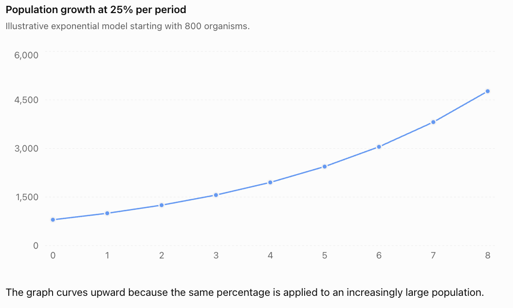
The graph curves upward because the same percentage is applied to an increasingly large population.

Comparing Linear and Exponential Growth

Linear and exponential growth may initially appear similar, but they behave differently over time.

Suppose two populations both begin with 1,000 individuals.

Population A increases by 200 individuals annually.

Population B increases by 20% annually.

Their models are:

Population A: Pₙ = 1,000 + 200n

Population B: Pₙ = 1,000(1.20)ⁿ

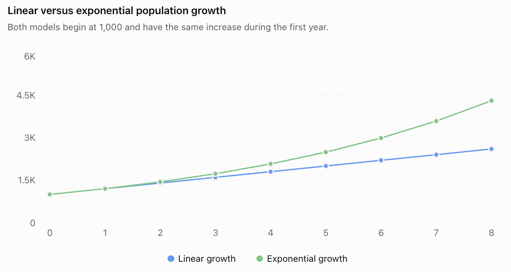
The linear population grows by the same number each year.

The exponential population grows by the same percentage each year.

This difference becomes increasingly important over longer time periods.

Population Decline and Exponential Decay

Populations can also decrease.

Decline may result from:

• Disease

• Habitat destruction

• Food shortages

• Predation

• Pollution

• Climate changes

• Emigration

• Overharvesting

If a population decreases by a constant percentage each period, it follows an exponential decay model.

Recursive model

Pₙ₊₁ = Pₙ(1 − r)

Explicit model

Pₙ = P₀(1 − r)ⁿ

where r is the decline rate as a decimal.

Worked Example 4: Wildlife Population Decline

A wildlife population contains 2,500 animals.

The population decreases by 8% annually.

Estimate the population after five years.

Step 1: Determine the decay factor.

1 − 0.08 = 0.92

Step 2: Write the model.

Pₙ = 2,500(0.92)ⁿ

Step 3: Calculate the population after five years.

P₅ = 2,500(0.92)⁵

≈ 2,500(0.6590815)

≈ 1,647.70

Answer: Approximately 1,648 animals

Interpreting exponential decay

The population decreases by 8% of its current size each year.

Therefore, the number of animals lost becomes smaller as the population becomes smaller.

An exponential decay model approaches zero mathematically but never reaches zero in a finite number of steps.

In reality, small populations may become extinct because populations consist of whole individuals and are affected by random events.

Half-Life and Population Decline

The half-life of a decreasing quantity is the time required for it to fall to half its initial value.

For exponential decay:

Pₙ = P₀(1 − r)ⁿ

At half-life:

Pₙ = P₀/2

Therefore:

1/2 = (1 − r)ⁿ

Taking logarithms:

n = ln(0.5)/ln(1 − r)

Worked Example 5: Population Half-Life

A population declines by 12% each year.

Estimate the time required for the population to fall to half its original size.

Decay factor:

0.88

Use:

n = ln(0.5)/ln(0.88)

≈ 5.42

Answer: Approximately 5.42 years

If the model is evaluated only at the end of each complete year, the population first falls below half its initial size after six years.

Half-life models also appear in radioactive decay, medicine, and environmental science.

Populations and Limited Resources

Exponential growth assumes that a population can continue increasing by the same percentage indefinitely.

In reality, populations depend on resources such as:

• Food

• Water

• Space

• Shelter

• Nutrients

• Suitable habitat

As population size increases, competition for these resources may become stronger.

Eventually, the environment may no longer support continued rapid growth.

The maximum population that an environment can sustain over a long period under particular conditions is called its carrying capacity.

Carrying capacity is usually represented by:

K

Understanding carrying capacity

The carrying capacity of an environment can change when resources or conditions change.

For example:

• Increased rainfall may raise carrying capacity.

• Habitat destruction may lower carrying capacity.

• Improved food availability may support more individuals.

• Disease or environmental disturbance may reduce the sustainable population.

Carrying capacity is not necessarily a fixed number.

Logistic Population Growth

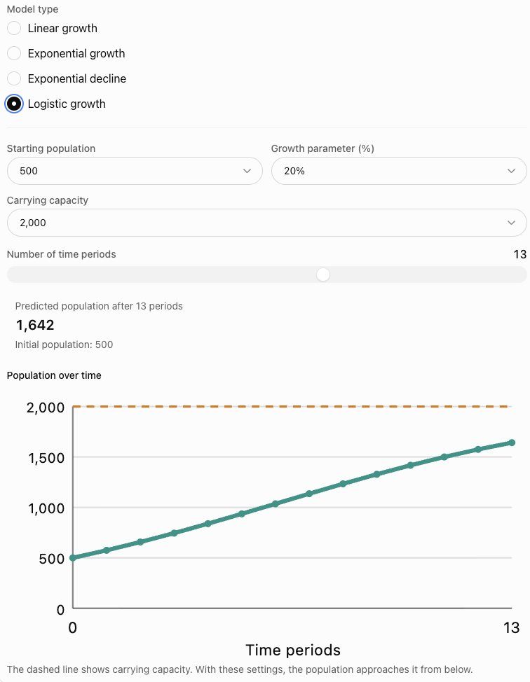
When resources are limited, population growth may slow as the population approaches carrying capacity.

This produces a logistic growth pattern.

A typical logistic curve has three stages:

1. Slow initial growth when the population is small.

2. Rapid growth when the population has sufficient resources.

3. Slowing growth as the population approaches carrying capacity.

The graph has an S-shaped appearance.

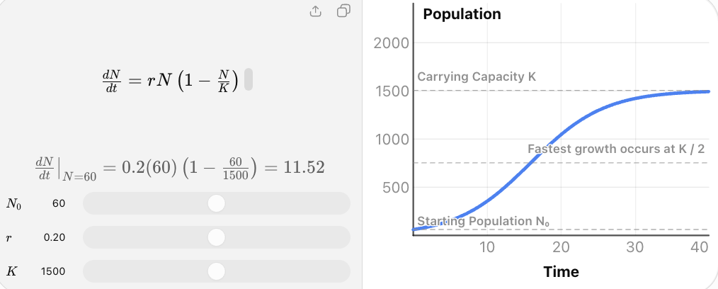
The logistic growth model is more realistic than unrestricted exponential growth in some environments because it includes the effect of limited resources.

A discrete logistic model

For populations measured at regular time intervals, one possible model is:

Pₙ₊₁ = Pₙ + rPₙ(1 − Pₙ/K)

where:

• Pₙ = population at time step n

• r = growth parameter per time step

• K = carrying capacity

The expression:

1 − Pₙ/K

reduces growth as the population approaches carrying capacity.

When Pₙ is much smaller than K, this factor is close to 1.

When Pₙ approaches K, this factor approaches 0.

The discrete model must be used carefully: depending on the growth parameter, it can produce oscillations or more complicated behaviour rather than smooth growth toward K.

Worked Example 6: Logistic Population Model

A fish population begins with 200 fish.

The lake has an estimated carrying capacity of 1,000 fish.

Use the recursive model:

Pₙ₊₁ = Pₙ + 0.4Pₙ(1 − Pₙ/1,000)

Find the population after two time periods.

Step 1: Initial population

P₀ = 200

Step 2: First period

P₁ = 200 + 0.4(200)(1 − 200/1,000)

= 200 + 80(0.8)

= 200 + 64

= 264

Step 3: Second period

P₂ = 264 + 0.4(264)(1 − 264/1,000)

= 264 + 105.6(0.736)

= 264 + 77.7216

= 341.7216

Answer: Approximately 342 fish

The population grows, but the growth term is reduced by the carrying-capacity factor.

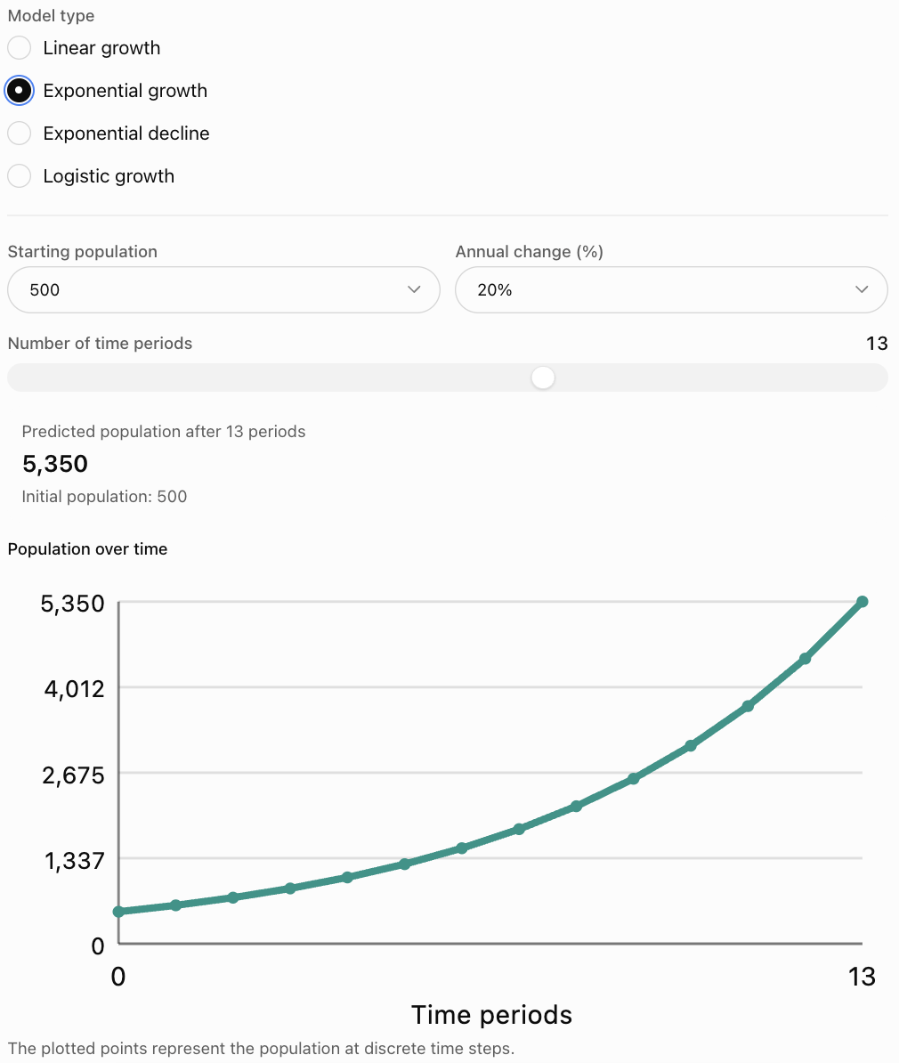
Interactive Population Model Explorer

Explore how a population changes under linear growth, exponential growth, exponential decline, and a discrete logistic model.

Resource Consumption Models

Population models are closely connected to resource models.

As populations grow, demand for resources may also increase.

Resources may include:

• Fresh water

• Food

• Energy

• Timber

• Fish stocks

• Agricultural land

• Minerals

• Fuel

Some resources are renewable, while others are non-renewable.

A mathematical model can help estimate how quickly resources are used and whether a resource supply is likely to remain sufficient.

Constant Resource Consumption

Suppose a reservoir contains 50,000 litres of water.

A community uses 2,000 litres each day, and no additional water enters the reservoir.

The remaining water forms an arithmetic sequence:

50,000, 48,000, 46,000, 44,000, ...

Recursive model

Rₙ₊₁ = Rₙ − c

where c is the amount consumed each period.

Explicit model

Rₙ = R₀ − nc

Worked Example 7: Water Consumption

A reservoir begins with 80,000 litres of water.

Water is consumed at a rate of 3,500 litres per day.

How much water remains after 15 days?

R₀ = 80,000

c = 3,500

n = 15

R₁₅ = 80,000 − 15(3,500)

= 80,000 − 52,500

Answer: 27,500 litres

When will the reservoir become empty?

Set:

80,000 − 3,500n = 0

3,500n = 80,000

n = 80,000/3,500

n ≈ 22.86

The reservoir would be exhausted during the 23rd day under this simplified model.

The formula should not be used to predict negative amounts of water after exhaustion.

Percentage-Based Resource Decline

Some resources decrease by a constant percentage during each period.

For example, suppose 15% of a stored material is lost each month through spoilage.

The remaining proportion is:

1 − 0.15 = 0.85

The recursive model is:

Rₙ₊₁ = 0.85Rₙ

The explicit model is:

Rₙ = R₀(0.85)ⁿ

Worked Example 8: Resource Decay

A storage facility begins with 10,000 kg of material.

Each month, 15% is lost.

How much remains after six months?

R₆ = 10,000(0.85)⁶

≈ 10,000(0.3771495)

Answer: Approximately 3,771.50 kg

Unlike constant consumption, the amount lost each month decreases as the remaining resource becomes smaller.

Renewable Resource Models

Renewable resources can recover naturally.

Examples include:

• Forests

• Fish populations

• Groundwater

• Agricultural crops

• Certain wildlife populations

A renewable resource model must consider both regeneration and consumption.

A simple model is:

Rₙ₊₁ = Rₙ + Gₙ − Hₙ

where:

• Rₙ = resource amount at time n

• Gₙ = resource regenerated during the period

• Hₙ = resource harvested or consumed during the period

Worked Example 9: Forest Regeneration

A forest contains 12,000 mature trees.

Each year:

• 800 trees reach maturity.

• 500 mature trees are harvested.

Assume these numbers remain constant.

The annual change is:

800 − 500 = 300 trees

Recursive model:

Rₙ₊₁ = Rₙ + 300

Explicit model:

Rₙ = 12,000 + 300n

After ten years:

R₁₀ = 12,000 + 300(10)

Answer: 15,000 mature trees

Evaluating the model

This model assumes that regeneration and harvesting remain constant.

Real forests are affected by rainfall, soil quality, disease, fire, land use, and the age structure of the trees.

A constant regeneration rate may be unrealistic over long periods.

Sustainable Harvesting and Resource Management

A resource is used sustainably when its use can be maintained over time without causing unacceptable long-term depletion.

In a simple model, resource quantity remains stable when:

Regeneration = Harvesting

For example, if a fish population produces a net increase of 400 fish annually and 400 fish are harvested annually, the population remains unchanged under those assumptions.

However, real ecosystems are more complex.

Harvesting can reduce the number of breeding individuals, which may reduce future regeneration.

Therefore, a sustainable harvesting model should account for how regeneration depends on population size.

Worked Example 10: Population with Harvesting

A fish population begins with 1,000 fish.

Each year, the population grows by 10%, after which 80 fish are harvested.

Write a recursive model and calculate the population after three years.

Step 1: Write the rule.

Pₙ₊₁ = 1.10Pₙ − 80

Step 2: Calculate the first year.

P₁ = 1.10(1,000) − 80

= 1,020

Step 3: Calculate the second year.

P₂ = 1.10(1,020) − 80

= 1,042

Step 4: Calculate the third year.

P₃ = 1.10(1,042) − 80

= 1,066.2

Answer: Approximately 1,066 fish

The population increases because the modelled growth exceeds harvesting during these years.

This does not prove that harvesting 80 fish annually would remain sustainable indefinitely. The model does not include carrying capacity or other ecological limits.

Predicting Future Population Sizes

Mathematical models allow us to estimate future values.

However, predictions become less reliable when the assumptions are uncertain.

Worked Example 11: Predicting City Population

A city has 150,000 residents.

Its population has recently grown by approximately 2% annually.

Estimate the population after 15 years if the same rate continues.

Use:

Pₙ = P₀(1 + r)ⁿ

Substitute:

P₁₅ = 150,000(1.02)¹⁵

≈ 150,000(1.345868)

Answer: Approximately 201,880 residents

Interpreting the prediction

This result does not guarantee that the city will have exactly 201,880 residents.

It represents the predicted population under the assumption that the annual growth rate remains at 2%.

Actual growth may be affected by housing, employment, migration, birth rates, and government policies.

Using Data to Select a Population Model

Before selecting a mathematical model, we should examine the available data.

Consider two datasets.

Dataset A

The differences are:

200, 200, 200, 200

This suggests a linear model:

Pₙ = 1,000 + 200n

Dataset B

The ratios are:

1.2, 1.2, 1.2, 1.2

This suggests an exponential model:

Pₙ = 1,000(1.2)ⁿ

Identifying the pattern

A constant difference suggests an arithmetic sequence.

A constant ratio suggests a geometric sequence.

Growth that slows as a population approaches an upper limit may suggest a logistic model.

Real data rarely follow an exact mathematical pattern, so model selection may require statistical analysis.

Evaluating the Limitations of Population Models

Mathematical models simplify real situations.

This makes them useful, but it also creates limitations.

1. Constant growth rates

An exponential model often assumes that the percentage growth rate remains unchanged.

Real growth rates may vary because of economic, biological, or environmental conditions.

2. Limited resources

Exponential growth ignores the effects of limited food, water, and space.

This may make long-term predictions unrealistic.

3. Random events

Disease outbreaks, natural disasters, and unexpected migration can cause sudden population changes.

Simple deterministic models do not capture these events.

4. Population structure

A population with many young individuals may behave differently from a population with many older individuals.

Simple models may ignore age and reproductive structure.

5. Environmental changes

Carrying capacity may change because of drought, pollution, climate change, or habitat restoration.

6. Incomplete or inaccurate data

Population estimates may contain measurement errors.

A model based on unreliable data may produce unreliable predictions.

7. Long-term extrapolation

A model that fits recent data may not remain accurate over many decades.

8. Fractional populations

Mathematical models may predict fractional individuals.

These values must be interpreted as estimates.

9. Human behaviour

Human population and resource use depend on economic decisions, policies, technology, and social changes.

These influences may be difficult to predict mathematically.

10. Model complexity

More complicated models may include additional variables and feedback mechanisms.

However, greater complexity does not automatically guarantee better predictions.

A good model balances mathematical usefulness with realistic assumptions.

Improving Population and Resource Models

Mathematical models can be improved by:

• Collecting more reliable data.

• Updating growth rates regularly.

• Including carrying capacity.

• Accounting for births, deaths, and migration separately.

• Incorporating resource regeneration and consumption.

• Considering seasonal changes.

• Comparing model predictions with actual observations.

• Using different scenarios to represent uncertainty.

Scenario analysis

Suppose a town currently has 20,000 residents.

We can examine three possible annual growth rates:

• Low growth: 1%

• Moderate growth: 2%

• High growth: 3%

After ten years:

Low-growth model:

P₁₀ = 20,000(1.01)¹⁰ ≈ 22,092

Moderate-growth model:

P₁₀ = 20,000(1.02)¹⁰ ≈ 24,380

High-growth model:

P₁₀ = 20,000(1.03)¹⁰ ≈ 26,878

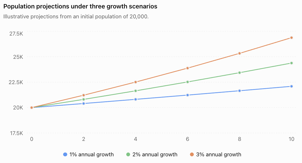
The difference between scenarios increases over time.

This demonstrates why small changes in growth rates can have significant long-term effects.

Real-World Applications

Common Mistakes

Mistake 1: Confusing constant growth with percentage growth

A population increasing by 100 each year is different from a population increasing by 10% each year.

Mistake 2: Using the percentage instead of the growth factor

For 8% growth, multiply by 1.08, not 0.08.

Mistake 3: Applying the wrong decay factor

A 12% decline means multiplying by 0.88.

Mistake 4: Forgetting the initial population

A recursive model requires a starting value.

Mistake 5: Using the wrong number of time periods

The number of periods must match the time interval used in the growth rate.

Mistake 6: Assuming exponential growth continues forever

Real populations are limited by resources and environmental conditions.

Mistake 7: Treating carrying capacity as permanently fixed

Carrying capacity can change over time.

Mistake 8: Confusing population growth with resource regeneration

Population growth and resource availability may follow different mathematical patterns.

Mistake 9: Predicting negative resource quantities

A resource model should be restricted to physically meaningful values.

Mistake 10: Rounding too early

Premature rounding can create errors in multi-step calculations.

Mistake 11: Assuming a mathematical prediction is guaranteed

Predictions depend on assumptions and may differ from actual outcomes.

Mistake 12: Ignoring uncertainty

Real-world population and resource models often require several possible scenarios.

Key Terms

• Population: Group of individuals of the same species living in a particular area.

• Population Model: Mathematical representation of changes in population size.

• Population Growth: Increase in the number of individuals over time.

• Population Decline: Decrease in the number of individuals over time.

• Birth Rate: Rate at which new individuals are born.

• Death Rate: Rate at which individuals die.

• Immigration: Movement of individuals into a population.

• Emigration: Movement of individuals out of a population.

• Arithmetic Sequence: Sequence with a constant difference.

• Geometric Sequence: Sequence with a constant ratio.

• Recursive Model: Model that calculates new values from previous values.

• Explicit Model: Formula that calculates a value directly from time or term number.

• Linear Growth: Growth by a constant amount per time period.

• Exponential Growth: Growth by a constant percentage per time period.

• Exponential Decay: Decline by a constant percentage per time period.

• Growth Factor: Multiplier representing percentage growth.

• Decay Factor: Multiplier representing percentage decline.

• Half-Life: Time required for a decreasing quantity to fall to half its original value.

• Carrying Capacity: Maximum population an environment can sustainably support under specified conditions.

• Logistic Growth: Growth that slows as a population approaches carrying capacity.

• Resource Model: Mathematical representation of resource availability or consumption.

• Renewable Resource: Resource that can naturally regenerate.

• Non-Renewable Resource: Resource that cannot be replenished on a relevant human timescale.

• Regeneration: Process through which a renewable resource is restored.

• Harvesting: Removal of individuals or resources for use.

• Sustainability: Ability to maintain a process or resource over time.

• Prediction: Estimated future value based on a model.

• Extrapolation: Using a model to predict values beyond the observed data.

• Assumption: Condition accepted when constructing a model.

• Limitation: Factor that restricts the accuracy or usefulness of a model.

• Scenario Analysis: Comparison of predictions under different assumptions.

Key Takeaways

• Population changes result from births, deaths, immigration, and emigration.

• Constant population increases produce arithmetic sequences.

• Constant percentage growth produces geometric sequences.

• Exponential growth can be modelled recursively or explicitly.

• Constant percentage decline produces exponential decay.

• Growth factors are greater than 1, while decay factors lie between 0 and 1.

• Real populations depend on limited environmental resources.

• Carrying capacity represents the population an environment can sustain under particular conditions.

• Logistic growth models account for slowing growth near carrying capacity.

• Resource consumption can be modelled using arithmetic or geometric sequences.

• Renewable resource models must consider both regeneration and consumption.

• Sustainable resource management requires understanding long-term population and resource changes.

• Mathematical models can predict future values but depend on assumptions.

• Model accuracy may decrease when predictions extend far beyond observed data.

• Comparing scenarios helps communicate uncertainty in population predictions.

Check Your Understanding

Questions

Question 1: Population Change

A town begins with 15,000 residents.

During one year:

• 500 people are born.

• 250 people die.

• 300 people move into the town.

• 400 people move away.

Calculate the final population.

Question 2: Arithmetic Population Growth

A village has 4,000 residents and gains 150 residents annually.

Write an explicit model and calculate the population after eight years.

Question 3: Geometric Population Growth

A population begins with 600 organisms and increases by 15% each year.

Write a recursive model.

Question 4: Predicting Population Growth

Using the population in Question 3, calculate the population after four years.

Question 5: Exponential Decline

A wildlife population contains 3,000 animals and decreases by 6% annually.

Estimate the population after five years.

Question 6: Identifying Models

Determine whether each sequence is arithmetic or geometric.

a) 200, 250, 300, 350, ...

b) 200, 250, 312.5, 390.625, ...

c) 1,000, 900, 810, 729, ...

Question 7: Half-Life

A population decreases by 10% annually.

Calculate the approximate time required for the population to fall to half its initial size.

Question 8: Carrying Capacity

Explain why exponential population growth cannot continue indefinitely in a natural ecosystem.

Question 9: Logistic Growth

A population is approaching its carrying capacity.

Describe how its growth rate is expected to change in a basic logistic model.

Question 10: Resource Consumption

A reservoir contains 120,000 litres of water.

A community uses 4,500 litres daily, and no new water enters.

Calculate the amount remaining after 20 days.

Question 11: Resource Decay

A storage facility contains 8,000 kg of material.

Each month, 5% is lost.

Calculate the amount remaining after six months.

Question 12: Renewable Resources

A forest begins with 10,000 mature trees.

Each year, 600 trees reach maturity and 450 are harvested.

Calculate the number of mature trees after eight years.

Question 13: Population and Harvesting

A fish population begins with 500 fish.

Each year, the population increases by 20%, after which 60 fish are harvested.

Write a recursive model and calculate the population after two years.

Question 14: Evaluating Models

Explain three limitations of using a constant percentage growth model to predict a wildlife population over 100 years.

Question 15: Integrated Challenge

A lake contains 1,200 fish.

The fish population increases by 12% annually, but 100 fish are harvested at the end of every year.

a) Write a recursive model.

b) Calculate the population after one year.

c) Calculate the population after two years.

d) Calculate the population after three years.

e) Explain whether this model is likely to remain realistic over a long period.

Fully Worked Answers

Answer 1: Population Change

Initial population:

15,000

Population change:

500 − 250 + 300 − 400

= 150

Final population:

15,000 + 150

Answer: 15,150 residents

Answer 2: Arithmetic Population Growth

Initial population:

P₀ = 4,000

Annual increase:

d = 150

Explicit model:

Pₙ = 4,000 + 150n

After eight years:

P₈ = 4,000 + 150(8)

= 4,000 + 1,200

Answer: 5,200 residents

Answer 3: Geometric Population Growth

Initial population:

P₀ = 600

Growth rate:

15% = 0.15

Growth factor:

1 + 0.15 = 1.15

Recursive model:

Pₙ₊₁ = 1.15Pₙ

Answer 4: Predicting Population Growth

Use:

Pₙ = 600(1.15)ⁿ

After four years:

P₄ = 600(1.15)⁴

≈ 600(1.74900625)

≈ 1,049.40

Answer: Approximately 1,049 organisms

Answer 5: Exponential Decline

Initial population:

P₀ = 3,000

Decline rate:

6%

Decay factor:

1 − 0.06 = 0.94

Model:

Pₙ = 3,000(0.94)ⁿ

After five years:

P₅ = 3,000(0.94)⁵

≈ 3,000(0.733904)

≈ 2,201.71

Answer: Approximately 2,202 animals

Answer 6: Identifying Models

Part a

200, 250, 300, 350, ...

Common difference:

50

Arithmetic sequence

Part b

200, 250, 312.5, 390.625, ...

Common ratio:

250/200 = 1.25

Geometric sequence

Part c

1,000, 900, 810, 729, ...

Common ratio:

900/1,000 = 0.90

Geometric decay sequence

Answer 7: Half-Life

Decay factor:

0.90

Use:

n = ln(0.5)/ln(0.90)

≈ 6.58

Answer: Approximately 6.58 years

For annual observations, the population first falls below half after seven complete years.

Answer 8: Carrying Capacity

Exponential growth assumes that a population can continue increasing by the same percentage.

Natural ecosystems have limited food, water, space, and other resources.

As population size increases, competition becomes stronger and growth may slow.

Therefore, exponential growth cannot continue indefinitely in a finite environment.

Answer 9: Logistic Growth

In a basic logistic model, population growth slows as the population approaches carrying capacity.

When the population is small relative to carrying capacity, growth may be relatively rapid.

As the population approaches carrying capacity, the growth rate in individuals per unit time decreases toward zero.

The population approaches a stable limiting value under suitable model conditions.

Answer 10: Resource Consumption

Initial resource:

R₀ = 120,000 litres

Daily consumption:

4,500 litres

Time:

20 days

Use:

Rₙ = R₀ − nc

R₂₀ = 120,000 − 20(4,500)

= 120,000 − 90,000

Answer: 30,000 litres

Answer 11: Resource Decay

Initial amount:

R₀ = 8,000 kg

Monthly loss:

5%

Decay factor:

0.95

Model:

Rₙ = 8,000(0.95)ⁿ

After six months:

R₆ = 8,000(0.95)⁶

≈ 8,000(0.7350919)

≈ 5,880.74

Answer: Approximately 5,881 kg

Answer 12: Renewable Resources

Initial number of mature trees:

10,000

Annual regeneration:

600

Annual harvesting:

450

Net annual change:

600 − 450 = 150

After eight years:

R₈ = 10,000 + 8(150)

= 10,000 + 1,200

Answer: 11,200 mature trees

Answer 13: Population and Harvesting

Initial population:

P₀ = 500

Growth rate:

20%

Annual harvest:

60

Recursive model:

Pₙ₊₁ = 1.20Pₙ − 60

First year:

P₁ = 1.20(500) − 60

= 600 − 60

= 540

Second year:

P₂ = 1.20(540) − 60

= 648 − 60

= 588

Answer: 588 fish

Answer 14: Evaluating Models

Three limitations are:

1. Limited resources

Food, water, and space may become insufficient as the population grows.

2. Environmental changes

Disease, drought, climate changes, and habitat destruction may alter growth rates.

3. Changing population structure

Birth and death rates may change as the population ages or its density changes.

Therefore, a constant percentage model may be useful for short-term predictions but unreliable over 100 years.

Answer 15: Integrated Challenge

Initial population:

P₀ = 1,200

Annual growth rate:

12%

Annual harvest:

100 fish

Part a: Recursive model

Pₙ₊₁ = 1.12Pₙ − 100

Part b: First year

P₁ = 1.12(1,200) − 100

= 1,344 − 100

P₁ = 1,244

Part c: Second year

P₂ = 1.12(1,244) − 100

= 1,393.28 − 100

P₂ = 1,293.28

Part d: Third year

P₃ = 1.12(1,293.28) − 100

= 1,448.4736 − 100

P₃ = 1,348.4736

Answer: Approximately 1,348 fish after three years

Part e: Evaluating the model

The model assumes that the population increases by 12% every year and that exactly 100 fish are harvested annually.

Over a long period, this may become unrealistic because:

• Food and space are limited.

• The lake has a finite carrying capacity.

• Reproduction and mortality may change.

• Environmental conditions may vary.

• Harvesting may affect the breeding population.

A more realistic long-term model might incorporate carrying capacity, variable growth rates, and environmental uncertainty.

Final Reflection

Population and resource models demonstrate how mathematical sequences can describe important processes in the natural world.

Arithmetic sequences help represent constant changes, while geometric sequences describe repeated percentage growth and decline. Recursive models allow us to account for births, deaths, harvesting, and resource regeneration.

More advanced models, such as logistic growth, help explain why populations cannot grow indefinitely in environments with limited resources.

Mathematical predictions are valuable for planning, conservation, and resource management, but they must always be interpreted in light of the assumptions used to construct them.

The most important lesson is that mathematical models help us understand population and resource changes, make predictions, and evaluate possible futures. However, a useful model must balance mathematical simplicity with the complexity of real-world systems.