5. Applications of Geometric Growth

Applications of Geometric Growth

Introduction

Geometric growth and decay occur when a quantity changes by the same multiplicative factor over equal intervals.

Unlike arithmetic growth, which involves adding a fixed amount, geometric growth involves multiplying by a fixed number.

For example, consider two populations that both begin with 100 organisms.

• Population A increases by 50 organisms each year.

• Population B increases by 50% each year.

After five years, the populations will be very different because one follows an arithmetic pattern while the other follows a geometric pattern.

Geometric relationships appear in many real-world situations, including population growth, compound interest, inflation, depreciation, radioactive decay, repeated discounts, and biological reproduction.

Understanding these patterns allows us to predict future values, compare alternatives, and calculate accumulated totals.

Recognising Geometric Growth and Decay

A geometric sequence has a constant ratio between consecutive terms.

Consider:

4, 8, 16, 32, 64, ...

Each term is multiplied by 2.

The common ratio is:

r = 2

This is geometric growth.

Now consider:

160, 80, 40, 20, 10, ...

Each term is multiplied by 0.5.

The common ratio is:

r = 0.5

This is geometric decay.

General Formula

For a sequence whose first term is at position n = 1:

aₙ = a₁rⁿ⁻¹

where:

• aₙ = value of the nth term

• a₁ = first term

• r = common ratio

• n = term number

For situations measured from an initial time of zero, a more convenient formula is:

A(t) = A₀rᵗ

where:

• A(t) = quantity after t time intervals

• A₀ = initial quantity

• r = multiplier per interval

• t = number of intervals elapsed

The formulas describe the same repeated-multiplication pattern, but use different starting positions.

Growth, Decay, and Constant Patterns

For populations, money balances, and many physical quantities, negative multipliers are usually not meaningful.

Converting Percentage Changes into Multipliers

Many geometric problems describe changes using percentages rather than common ratios.

The first step is to convert the percentage into a decimal multiplier.

Percentage Increase

For an increase of p%:

Growth multiplier = 1 + p/100

Examples:

A 25% increase means the new value is 125% of the previous value.

Therefore:

New value = Previous value × 1.25

Percentage Decrease

For a decrease of p%:

Decay multiplier = 1 − p/100

Examples:

A 20% decrease means the new value is 80% of the previous value.

Therefore:

New value = Previous value × 0.80

Worked Example

A quantity increases by 12% each year.

Find the multiplier.

r = 1 + 12/100

r = 1 + 0.12

r = 1.12

If the quantity starts at 500:

A(t) = 500(1.12)ᵗ

This formula models a 12% increase every year.

Modelling Population Growth

Population growth is one of the most common applications of geometric sequences.

Under ideal conditions, some populations increase by approximately the same percentage during each time interval.

Examples include:

• Bacterial reproduction.

• Insect populations.

• Plant populations during favourable growing conditions.

• Introduced species during early population expansion.

Worked Example: Bacterial Growth

A bacterial culture begins with 200 cells.

The population doubles every hour.

Step 1: Identify the Initial Population

P₀ = 200 cells

Step 2: Identify the Multiplier

The population doubles.

r = 2

Step 3: Write the Formula

P(t) = 200 × 2ᵗ

where t is the number of hours elapsed.

Step 4: Create a Table

Step 5: Predict the Population After Eight Hours

P(8) = 200 × 2⁸

P(8) = 200 × 256

P(8) = 51,200 cells

Interpretation

The population doubles every hour, so the number of new cells produced during each hour increases as the population grows.

The increase from 200 to 400 is only 200 cells.

The increase from 6,400 to 12,800 is 6,400 cells.

The percentage growth remains constant even though the numerical increase becomes larger.

Population Growth Using Percentages

Not all populations double or triple.

Some increase by smaller percentages.

Worked Example

A town has an initial population of 12,000 people.

Its population grows by 3% each year.

Estimate the population after five years.

Step 1: Identify the Initial Population

P₀ = 12,000

Step 2: Convert the Percentage

r = 1 + 0.03

r = 1.03

Step 3: Write the Model

P(t) = 12,000(1.03)ᵗ

Step 4: Substitute t = 5

P(5) = 12,000(1.03)⁵

P(5) ≈ 12,000 × 1.159274

P(5) ≈ 13,911 people

Interpretation

The model predicts approximately 13,911 people after five years.

Because population is counted in whole people, we round the result to the nearest whole number.

Limitations of Population Models

Real populations do not necessarily grow geometrically forever.

Growth can be affected by:

• Food and water availability.

• Disease.

• Competition.

• Migration.

• Predation.

• Birth and death rates.

• Environmental conditions.

Geometric models are often most useful over periods when the percentage growth rate is reasonably stable.

When resources become limited, population growth may slow and approach a carrying capacity rather than continuing exponentially.

Understanding Compound Interest

Compound interest is another important application of geometric growth.

When money earns compound interest, interest is calculated on the current balance, including interest earned during previous periods.

This creates repeated multiplication.

Simple Interest Versus Compound Interest

Suppose $1,000 earns 10% interest annually.

With simple interest, the same $100 is added each year.

With compound interest, each year earns 10% of the updated balance.

Simple interest follows an arithmetic pattern.

Compound interest follows a geometric pattern.

Why Does Compound Interest Grow Faster?

With compound interest, the interest earned becomes part of the balance used to calculate future interest.

This is sometimes described as earning interest on interest.

Compound Interest Formula

For an initial investment with a fixed interest rate compounded once per period:

FV = PV(1 + i)ⁿ

where:

• FV = future value

• PV = present value or initial investment

• i = interest rate per compounding period, expressed as a decimal

• n = number of compounding periods

This is a geometric model with multiplier:

r = 1 + i

Worked Example: Investment Growth

An investor deposits $2,500 into an account earning 6% annual interest, compounded annually.

Calculate the balance after eight years.

Step 1: Identify the Values

PV = $2,500

i = 0.06

n = 8

Step 2: Substitute

FV = 2,500(1.06)⁸

Step 3: Calculate

(1.06)⁸ ≈ 1.593848

FV ≈ 2,500 × 1.593848

FV ≈ $3,984.62

Step 4: Calculate the Interest Earned

Interest = Final balance − Initial investment

Interest = 3,984.62 − 2,500

Interest earned ≈ $1,484.62

Interpretation

The account grows because each year's interest is calculated using the balance accumulated during the previous years.

This model assumes a fixed interest rate, no additional deposits or withdrawals, and no fees or taxes.

How Compounding Frequency Changes Growth

Interest may be compounded annually, semiannually, quarterly, monthly, or daily.

When a nominal annual interest rate is divided into multiple compounding periods, the formula becomes:

A = P(1 + i/m)ᵐᵗ

where:

• P = initial principal

• i = nominal annual interest rate

• m = number of compounding periods per year

• t = time in years

Worked Example

An investment of $1,000 earns 12% nominal annual interest, compounded monthly.

Find its value after one year.

P = 1,000

i = 0.12

m = 12

t = 1

Substitute:

A = 1,000(1 + 0.12/12)¹²

A = 1,000(1.01)¹²

A ≈ $1,126.83

The investment earns approximately $126.83 in interest.

This is slightly more than the $120 earned if 12% interest were compounded only once at the end of the year.

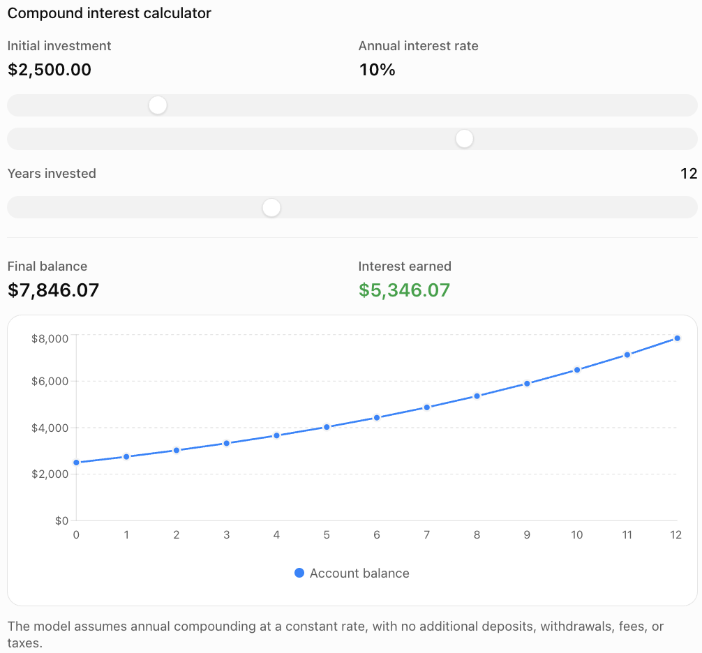
Exploring Compound Interest

The following model allows you to explore how the initial investment, interest rate, and number of periods affect compound growth.

What Can We Learn?

Changing the initial investment changes the starting value.

Changing the interest rate changes the common ratio.

Changing the number of years changes how many times the balance is multiplied.

Even a small change in the interest rate can produce a significant difference over long periods.

Geometric Decay and Depreciation

Geometric relationships also describe situations in which a quantity decreases by a fixed percentage during each interval.

Depreciation is a decrease in an asset's value over time.

For example, a vehicle may lose a percentage of its remaining value each year.

Worked Example: Vehicle Depreciation

A vehicle is purchased for $30,000.

Its value decreases by 15% each year.

Find its estimated value after four years.

Step 1: Identify the Initial Value

V₀ = $30,000

Step 2: Calculate the Multiplier

r = 1 − 0.15

r = 0.85

Step 3: Write the Formula

V(t) = 30,000(0.85)ᵗ

Step 4: Calculate

V(4) = 30,000(0.85)⁴

V(4) = 30,000 × 0.52200625

V(4) ≈ $15,660.19

Step 5: Calculate the Total Depreciation

30,000 − 15,660.19 = 14,339.81

Total depreciation ≈ $14,339.81

Interpretation

The vehicle loses 15% of its remaining value each year, not 15% of its original purchase price.

Therefore, the amount lost in dollars becomes smaller over time.

Actual resale values may differ from this simplified model.

Repeated Percentage Changes

Geometric models are especially useful when percentages are applied repeatedly.

Worked Example: Repeated Discounts

A jacket originally costs $200.

The store reduces its price by 20%, then applies an additional 10% discount.

First Discount

200 × 0.80 = 160

New price = $160

Second Discount

160 × 0.90 = 144

Final price = $144

Overall Discount

200 − 144 = 56

56/200 × 100% = 28%

The total discount is 28%, not 30%.

Why?

The second discount is applied to the already reduced price.

Repeated percentage changes must be multiplied, not simply added.

The combined multiplier is:

0.80 × 0.90 = 0.72

Therefore, the jacket retains 72% of its original price.

Another Example: Increase Followed by Decrease

A product increases in price by 20%, then decreases by 20%.

The combined multiplier is:

1.20 × 0.80 = 0.96

The final price is 96% of the original price.

The overall change is a 4% decrease.

Equal percentage increases and decreases do not cancel each other because they are applied to different starting values.

Geometric Series in Real-World Problems

So far, we have used geometric sequences to find individual values.

However, many practical problems require the sum of several values.

A geometric series adds the terms of a geometric sequence.

For example:

5 + 10 + 20 + 40 + 80

The corresponding sequence has:

a₁ = 5

r = 2

The sum is:

5 + 10 + 20 + 40 + 80 = 155

Therefore:

S₅ = 155

Finite Geometric Series Formula

For r ≠ 1:

Sₙ = a₁(1 − rⁿ)/(1 − r)

An equivalent form is:

Sₙ = a₁(rⁿ − 1)/(r − 1)

where:

• Sₙ = sum of the first n terms

• a₁ = first term

• r = common ratio

• n = number of terms

If r = 1, every term is equal and:

Sₙ = na₁

Why Does the Formula Work?

Consider:

Sₙ = a₁ + a₁r + a₁r² + ... + a₁rⁿ⁻¹

Multiply by r:

rSₙ = a₁r + a₁r² + ... + a₁rⁿ

Subtract the second expression from the first:

Sₙ − rSₙ = a₁ − a₁rⁿ

Factor:

Sₙ(1 − r) = a₁(1 − rⁿ)

Divide by 1 − r:

Sₙ = a₁(1 − rⁿ)/(1 − r)

The formula works because the middle terms cancel during subtraction.

Application: Total Savings

A student saves $10 during the first week and doubles the amount saved each following week.

How much will the student save over eight weeks?

Step 1: Identify the Values

a₁ = 10

r = 2

n = 8

Step 2: Write the Formula

S₈ = 10(2⁸ − 1)/(2 − 1)

Step 3: Calculate

S₈ = 10(256 − 1)

S₈ = 10 × 255

S₈ = $2,550

Verification

The weekly savings are:

10, 20, 40, 80, 160, 320, 640, 1,280

Adding them gives:

$2,550

Interpretation

The eighth week's savings are $1,280.

The total savings over eight weeks are $2,550.

This illustrates the difference between a geometric sequence term and a geometric series sum.

Application: Regular Contributions to an Investment

Geometric series can also model a series of deposits that earn compound interest.

Suppose a person deposits $100 at the end of each year into an account earning 5% annually.

At the end of the fourth year, the deposits have the following values:

The total value is:

FV = 100(1.05)³ + 100(1.05)² + 100(1.05) + 100

FV = 115.7625 + 110.25 + 105 + 100

FV ≈ $431.01

The deposits form a geometric series when their values are measured at the same future date.

Important Distinction

A single initial deposit follows a geometric growth model.

A series of equal deposits can produce a geometric series when we calculate their accumulated future values.

Application: Bouncing Balls and Total Distance

A ball is dropped from a height of 8 metres.

After each bounce, it rises to 60% of its previous maximum height.

Step 1: Calculate the Rebound Heights

First rebound:

8 × 0.6 = 4.8 m

Second rebound:

4.8 × 0.6 = 2.88 m

Third rebound:

2.88 × 0.6 = 1.728 m

Fourth rebound:

1.728 × 0.6 = 1.0368 m

Step 2: Find the Total of the Rebound Heights

4.8 + 2.88 + 1.728 + 1.0368

= 10.4448 m

Step 3: Calculate the Total Distance

The initial drop is 8 metres.

Each complete rebound includes upward and downward motion.

Total distance through four complete rebounds:

D = 8 + 2(10.4448)

D = 28.8896 m

Interpretation

The ball travels approximately 28.89 metres by the time it returns to the ground after the fourth rebound.

The total distance is greater than the initial drop height because the ball repeatedly travels upward and downward.

Application: Radioactive Decay

Radioactive decay can be modelled using a geometric relationship when we measure the expected remaining quantity at equal intervals.

The half-life is the time required for half of a large sample's undecayed radioactive nuclei to decay, on average.

Worked Example

A radioactive sample initially contains 640 mg of an isotope.

Its half-life is 5 years.

Find the expected remaining mass after 20 years.

Step 1: Identify the Number of Half-Lives

20/5 = 4

Step 2: Identify the Multiplier

r = 0.5

Step 3: Write the Model

M = 640(0.5)ⁿ

where n is the number of completed half-life intervals.

Step 4: Calculate

M(4) = 640(0.5)⁴

M(4) = 640/16

M(4) = 40 mg

Interpretation

The model predicts that approximately 40 mg remains after 20 years.

The mass decreases geometrically because the expected remaining quantity is multiplied by 0.5 after every half-life.

Comparing Arithmetic and Geometric Growth

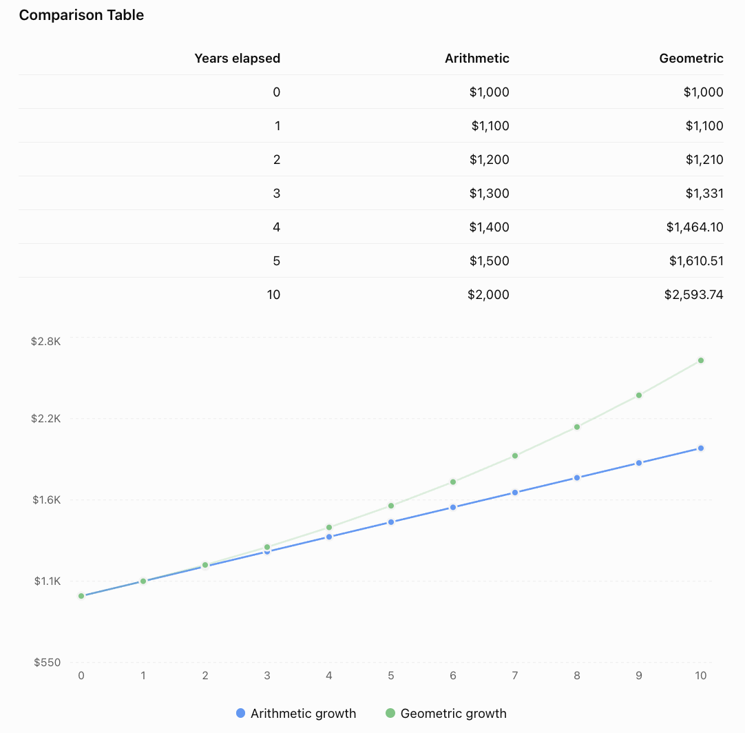
Suppose two investments begin at $1,000.

Investment A increases by $100 each year.

Investment B increases by 10% each year.

Arithmetic Model

A(t) = 1,000 + 100t

Geometric Model

B(t) = 1,000(1.10)ᵗ

Interpretation

The arithmetic model increases by a constant dollar amount.

The geometric model increases by a constant percentage.

Because the geometric model calculates growth from an increasing balance, its dollar increases become larger each year.

Choosing the Correct Mathematical Model

Not every situation involving change is geometric.

The key is identifying how the quantity changes.

Questions to Ask

When deciding which model to use, ask:

1. Does the quantity change by a constant amount or a constant percentage?

2. Is the change additive or multiplicative?

3. What is the starting value?

4. What is the common difference or common ratio?

5. What time interval does each step represent?

6. Are we finding an individual value or an accumulated total?

7. Is the model realistic over the required time period?

Common Mistakes

Adding a percentage instead of multiplying

A 10% increase means multiplying by 1.10, not adding 10 to the quantity.

Using the percentage as the multiplier

A 15% increase uses r = 1.15, not r = 0.15.

Using the wrong decay factor

A 20% decrease uses r = 0.80, not r = 0.20.

Confusing a sequence term with a series sum

A term represents one value. A series sum represents the total of several values.

Confusing the starting time

For models beginning at time zero, use an exponent of t. For sequences indexed from term one, use n − 1.

Adding repeated percentage changes

Successive percentage changes should be represented by multiplying their factors.

Rounding too early

Keep several decimal places during calculations and round the final answer appropriately.

Assuming geometric growth continues indefinitely

Real populations, investments, and physical systems may experience changing conditions.

Confusing simple and compound interest

Simple interest uses a fixed amount of interest each period. Compound interest uses the updated balance.

Using inconsistent time units

The multiplier and exponent must refer to the same interval. A monthly multiplier must be used with a number of months.

Key Terms

• Geometric Growth: Increase caused by repeated multiplication by a constant factor greater than 1.

• Geometric Decay: Decrease caused by repeated multiplication by a factor between 0 and 1.

• Geometric Sequence: Sequence with a constant ratio between consecutive terms.

• Geometric Series: Sum of terms from a geometric sequence.

• Common Ratio: Fixed multiplier between consecutive terms.

• Growth Factor: Multiplier used to represent a percentage increase.

• Decay Factor: Multiplier used to represent a percentage decrease.

• Initial Value: Quantity at the beginning of a model.

• Exponential Growth: Growth described by repeated multiplication.

• Exponential Decay: Decay described by repeated multiplication.

• Compound Interest: Interest calculated using the current balance, including previously earned interest.

• Simple Interest: Interest calculated only on the original principal.

• Principal: Initial amount invested or borrowed.

• Future Value: Value of an investment at a later time.

• Depreciation: Decrease in an asset's value over time.

• Inflation: General increase in prices over time.

• Half-Life: Time required for half of a radioactive sample's undecayed nuclei to decay on average.

• Partial Sum: Sum of a specified number of terms.

• Finite Geometric Series: Sum of a fixed number of geometric terms.

• Mathematical Model: Mathematical representation of a real-world process.

• Carrying Capacity: Maximum population an environment can sustainably support under given conditions.

• Accumulation: Building a total through repeated contributions.

• Percentage Change: Change expressed relative to the previous value.

Key Takeaways

• Geometric growth and decay involve repeated multiplication.

• A constant percentage change produces a geometric pattern.

• The multiplier for a p% increase is 1 + p/100.

• The multiplier for a p% decrease is 1 − p/100.

• Geometric sequences can model population growth, compound interest, and depreciation.

• The formula aₙ = a₁rⁿ⁻¹ calculates individual terms of a geometric sequence.

• The formula A(t) = A₀rᵗ models changes from an initial time of zero.

• Compound interest produces geometric growth because interest is calculated on the updated balance.

• Geometric series calculate accumulated totals.

• The finite geometric series formula is Sₙ = a₁(1 − rⁿ)/(1 − r), when r ≠ 1.

• Repeated percentage changes must be multiplied, not added.

• Arithmetic models involve constant amounts; geometric models involve constant ratios.

• Real-world models depend on assumptions and may not remain accurate indefinitely.

Check Your Understanding

Identifying Geometric Patterns

1. Explain the difference between arithmetic and geometric growth.

2. Determine the multiplier for a 12% increase.

3. Determine the multiplier for a 25% decrease.

4. Is a salary increase of $200 per year arithmetic or geometric?

5. Is a population increase of 8% per year arithmetic or geometric?

Population Growth

6. A population begins with 500 organisms and doubles each year. Write a formula for its population after t years.

7. Find the population after four years.

8. A town has 10,000 residents and grows by 2% annually. Write a geometric model.

9. Estimate its population after three years.

Compound Interest

10. An investment of $1,000 earns 5% compound interest annually. Write the growth formula.

11. Find its balance after three years.

12. Explain why compound interest produces geometric growth.

13. Explain the difference between simple and compound interest.

Repeated Percentage Changes

14. A product costs $100 and decreases in price by 20%. Find its new price.

15. The reduced price decreases by another 20%. Find the final price.

16. Explain why two successive 20% discounts do not produce a 40% discount.

Geometric Series

17. Calculate 5 + 10 + 20 + 40 + 80.

18. A student saves $10, $20, $40, and $80 over four weeks. Find the total.

19. Find the sum of the first five terms of 3, 6, 12, 24, ...

20. Explain the difference between a geometric sequence and a geometric series in a savings problem.

Answer Key

Extended Challenge

Growth and Decay Models

1. A population of 800 organisms grows by 15% annually. Write a formula and calculate the population after six years.

2. A bacterial culture begins with 150 cells and triples every two hours. Estimate the population after eight hours.

3. A city begins with 50,000 residents and grows by 1.8% annually. Estimate its population after ten years.

4. A vehicle worth $45,000 loses 12% of its value annually. Calculate its value after six years.

5. A radioactive sample initially contains 1,280 mg and has a half-life of four years. Calculate its expected remaining mass after 16 years.

Financial Applications

6. An investment of $5,000 earns 7% annual compound interest. Find its value after ten years.

7. Compare $2,000 invested for five years at 5% simple interest and 5% compound interest.

8. A product increases in price by 15%, then decreases by 10%. Determine the overall percentage change.

9. A computer costs $1,500 and depreciates by 20% annually. Find its estimated value after four years.

10. An investment earns 4% annually. Determine how many complete years are required for its balance to first exceed 150% of its initial value.

Geometric Series

11. A student saves $5 in the first week and doubles the amount saved each week. Find the total saved over ten weeks.

12. A theatre display contains 3 lights in its first row and twice as many in each successive row. Find the total lights in the first eight rows.

13. A ball rebounds to 80% of its previous height. If dropped from 10 metres, find the sum of its first five rebound heights.

14. Find the sum of the first six terms of 4, 12, 36, 108, ...

15. A company awards bonuses of $100, $150, $225, and $337.50. Find the total amount awarded.

Analysis and Evaluation

16. Explain why population growth cannot continue exponentially forever.

17. Compare the graphs of arithmetic and geometric growth.

18. Explain why a 50% increase followed by a 50% decrease does not return a quantity to its original value.

19. Describe a real-world situation in which a geometric series is more useful than a geometric sequence.

20. Explain why identifying the correct time interval is essential when applying geometric models.

Final Investigation: Planning a Savings Strategy

Two students begin saving money.

Student A saves $20 during the first week and increases the amount saved by $10 each following week.

Student B saves $20 during the first week and increases the amount saved by 25% each following week.

Complete the investigation.

1. Identify which savings plan follows an arithmetic sequence.

2. Identify which savings plan follows a geometric sequence.

3. Determine the common difference for Student A.

4. Determine the common ratio for Student B.

5. Write the nth term formula for each savings plan.

6. Calculate the amount each student saves during Week 5.

7. Calculate the amount each student saves during Week 10.

8. Create a table of weekly savings for the first ten weeks.

9. Graph the two sequences on the same coordinate plane.

10. Calculate the total savings for Student A over ten weeks.

11. Calculate the total savings for Student B over ten weeks.

12. Determine which student has saved more after ten weeks.

13. Explain why the geometric plan may eventually produce much larger weekly savings.

14. Identify the first week in which Student B's weekly savings exceed Student A's.

15. Discuss whether both savings plans are realistic over a long period.

16. Explain the difference between the weekly savings and total savings.

17. Predict how changing Student B's growth rate to 10% would affect the results.

18. Predict how changing Student A's weekly increase to $20 would affect the results.

19. Describe which plan you would prefer for a short savings period and explain your reasoning.

20. Explain how geometric sequences and series help people make financial decisions.