5. Modeling Relationships

Modeling Relationships

Introduction

Mathematics is not only about calculating answers. It is also about finding patterns, describing relationships, and using those relationships to understand the world.

A mathematical model is a mathematical representation of a real-world situation. Models can take the form of equations, tables, graphs, diagrams, or formulas.

For example, we can use mathematical models to:

• Calculate the cost of buying several items.

• Predict how far a vehicle will travel.

• Estimate the amount of water in a tank.

• Compare different mobile phone plans.

• Calculate earnings from working a certain number of hours.

• Predict the growth of a population.

• Determine whether a business is making a profit.

An algebraic model allows us to describe how one quantity depends on another and make predictions without calculating every possible value individually.

What Is a Mathematical Model?

A mathematical model uses mathematics to represent a situation or relationship.

A model may be an equation, graph, table, or other mathematical representation.

Example

A notebook costs $3.

If n represents the number of notebooks purchased and C represents the total cost, then:

C = 3n

This equation is a mathematical model.

It describes how the total cost changes with the number of notebooks purchased.

Using the Model

If 5 notebooks are purchased:

C = 3(5)

C = $15

If 12 notebooks are purchased:

C = 3(12)

C = $36

Important Observation

A useful mathematical model allows us to calculate unknown values and make predictions.

However, a model is only reliable when its assumptions match the real situation.

Understanding Variables

A variable is a symbol representing a quantity that can change or is unknown.

In mathematical models, variables often describe quantities that depend on one another.

Independent Variable

The independent variable is the input quantity.

It is usually represented by x.

Dependent Variable

The dependent variable is the output quantity.

It is usually represented by y.

Example

A worker earns $18 per hour.

Let:

• h = number of hours worked

• E = total earnings in dollars

The model is:

E = 18h

The number of hours worked is the independent variable.

The total earnings are the dependent variable.

Important Observation

The dependent variable changes according to the value of the independent variable.

Creating Algebraic Rules from Words

Real-world situations can often be translated into algebraic equations.

Common Mathematical Language

Worked Example

A swimming pool charges a $6 entrance fee plus $2 for each hour spent swimming.

Let:

h = number of hours

C = total cost

Step 1: Identify the Fixed Amount

Entrance fee = $6

Step 2: Identify the Variable Amount

Hourly charge = $2

Step 3: Write the Equation

C = 2h + 6

Step 4: Interpret

The total cost begins at $6 and increases by $2 for every additional hour.

Recognising Relationships from Tables

Tables can reveal patterns that help us construct algebraic rules.

Example

Step 1: Find the Pattern

The output increases by 3 whenever the input increases by 1.

Therefore, the rate of change is 3.

Step 2: Find the Initial Value

When x = 0:

y = 4

The initial value is 4.

Step 3: Write the Rule

y = 3x + 4

Step 4: Verify

When x = 4:

y = 3(4) + 4

y = 16

The rule matches the table.

Important Observation

A constant rate of change suggests a linear relationship.

Linear Mathematical Models

A linear model has the general form:

y = mx + b

where:

• m = constant rate of change

• b = initial value

Example

A taxi charges $5 to begin a journey and $2 per kilometre.

The model is:

C = 2d + 5

where:

• C = total cost in dollars

• d = distance in kilometres

Interpretation

• The slope is 2, representing $2 per kilometre.

• The initial value is 5, representing the starting fee.

Predicting Cost

For a 12 km journey:

C = 2(12) + 5

C = 24 + 5

C = $29

Important Observation

Linear models are appropriate when the rate of change remains constant.

Visualising a Linear Model

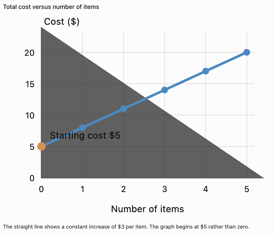
Consider the model:

C = 3x + 5

This could represent a $5 fixed fee plus $3 for each item.

Direct Variation Models

Some relationships are directly proportional.

A direct variation model has the form:

y = kx

where k is the constant of proportionality.

Example

A machine produces 25 items per minute.

Let:

P = number of items produced

t = time in minutes

The model is:

P = 25t

Predicting Production

After 8 minutes:

P = 25(8)

P = 200 items

Important Observation

A direct variation graph passes through the origin because the output is zero when the input is zero.

Comparing Direct Variation and General Linear Models

Example

Buying pencils at $2 each:

C = 2n

This is direct variation.

Buying pencils at $2 each with a $5 delivery fee:

C = 2n + 5

This is linear but not directly proportional.

Creating Models from Two Data Points

Sometimes we are given two observations rather than an equation.

If a linear relationship is appropriate, two points with different x-values determine the equation.

Worked Example

A water tank contains 120 litres after 2 minutes and 200 litres after 6 minutes.

Assume water enters at a constant rate.

Step 1: Identify the Points

(2, 120)

(6, 200)

Step 2: Calculate the Rate of Change

m = (200 − 120)/(6 − 2)

m = 80/4

m = 20 L/min

Step 3: Write the General Equation

V = 20t + b

Step 4: Find the Initial Volume

Use (2, 120):

120 = 20(2) + b

120 = 40 + b

b = 80

Final Model

V = 20t + 80

Interpretation

The tank initially contained 80 litres and gains 20 litres per minute.

Using Models to Make Predictions

Once a mathematical model has been constructed, it can be used to predict unknown values.

Worked Example

A company charges $15 per month plus $0.10 per text message.

The model is:

C = 15 + 0.10n

where n is the number of text messages.

Predict the Cost of 120 Messages

C = 15 + 0.10(120)

C = 15 + 12

C = $27

Determine the Number of Messages for a $35 Bill

35 = 15 + 0.10n

20 = 0.10n

n = 200 messages

Important Observation

A mathematical model can be used to find either the input or the output, depending on the information given.

Interpreting the Meaning of Slope

The slope describes how quickly one quantity changes relative to another.

Example

A tank loses 12 litres of water per minute.

The volume is modelled by:

V = 300 − 12t

where:

• V = volume in litres

• t = time in minutes

The slope is −12.

Interpretation

The negative slope indicates that the volume decreases by 12 litres every minute.

Prediction

After 10 minutes:

V = 300 − 12(10)

V = 180

180 litres remain.

Important Observation

A negative slope represents a decreasing relationship.

Interpreting the Initial Value

The initial value represents the output when the input is zero.

Example

A savings account begins with $250.

A person deposits $40 every week.

The model is:

S = 40w + 250

where:

• S = savings in dollars

• w = number of weeks

Interpretation

• Slope = 40 dollars per week.

• Initial value = $250.

Prediction

After 12 weeks:

S = 40(12) + 250

S = 480 + 250

S = $730

Important Observation

The initial value often represents a starting amount, fixed fee, or initial measurement.

Modeling Relationships in Shopping

Shopping situations often involve constant unit prices and fixed charges.

Worked Example

A store sells notebooks for $4 each and charges $6 for delivery.

Step 1: Define Variables

n = number of notebooks

C = total cost

Step 2: Write the Model

C = 4n + 6

Step 3: Predict the Cost of 15 Notebooks

C = 4(15) + 6

C = 60 + 6

C = $66

Step 4: Evaluate the Model

The model assumes:

• Each notebook costs $4.

• Delivery always costs $6.

• No discounts apply.

• No additional taxes or charges apply.

If any assumption changes, the model may need to be revised.

Modeling Relationships in Transportation

Transportation provides many examples of mathematical modeling.

Worked Example

A taxi company charges:

• $4 starting fee

• $2.50 per kilometre

Equation

C = 2.5d + 4

Prediction

For a 16 km journey:

C = 2.5(16) + 4

C = 40 + 4

C = $44

Model Limitations

The model may not account for:

• Waiting time.

• Traffic surcharges.

• Toll roads.

• Different rates at night.

• Special discounts.

Important Observation

A mathematical model simplifies reality by focusing on selected variables.

Modeling Relationships in Science

Mathematical models are widely used in science.

Example: Constant-Speed Motion

If an object travels at constant speed:

d = vt

where:

• d = distance

• v = speed

• t = time

Worked Example

A cyclist travels at 18 km/h.

The model is:

d = 18t

After 2.5 hours:

d = 18(2.5)

d = 45 km

Evaluating the Model

The model assumes constant speed.

In reality, the cyclist may:

• Stop for breaks.

• Travel uphill or downhill.

• Encounter traffic.

• Change speed due to fatigue.

The model is useful for estimating distance but may not describe every moment of the journey accurately.

Modeling Temperature Changes

Some temperature changes can be approximated by linear models over short periods.

Example

A liquid begins at 80°C and cools by approximately 3°C per minute during a short observation period.

The model is:

T = 80 − 3t

where:

• T = temperature in °C

• t = time in minutes

Prediction

After 5 minutes:

T = 80 − 3(5)

T = 65°C

Evaluating the Model

The model may work over the measured interval.

However, real cooling often slows as the liquid approaches room temperature.

Therefore, the model should not be assumed accurate indefinitely.

Important Observation

A model can be useful over a limited range even if it does not describe the entire process perfectly.

Comparing Mathematical Models

Sometimes two different equations describe competing choices.

Worked Example

Two internet providers offer different monthly plans.

Provider A:

C = 5d + 20

Provider B:

C = 3d + 36

where d represents additional data usage in GB and C represents the monthly cost in dollars.

Step 1: Compare Initial Costs

Provider A starts at $20.

Provider B starts at $36.

Step 2: Compare Rates

Provider A charges $5 per GB.

Provider B charges $3 per GB.

Step 3: Find Equal Costs

5d + 20 = 3d + 36

2d = 16

d = 8 GB

Step 4: Calculate the Common Cost

C = 5(8) + 20

C = $60

Interpretation

• Below 8 GB, Provider A is cheaper.

• At 8 GB, both cost $60.

• Above 8 GB, Provider B is cheaper.

Important Observation

Comparing models allows us to identify the best option under different conditions.

Recognising When a Linear Model Is Appropriate

A linear model is useful when the rate of change is constant.

Example: Linear Data

The volume increases by 15 litres each minute.

The model is:

V = 15t + 20

Example: Nonlinear Data

The output doubles each time.

The differences are not constant.

Therefore, a linear model is not appropriate.

This pattern can be represented by:

y = 2 × 2ˣ

Important Observation

A model should be selected based on the behaviour of the data, not simply because an equation is easy to use.

Evaluating Whether a Model Fits the Data

A mathematical model should be compared with real observations.

Example

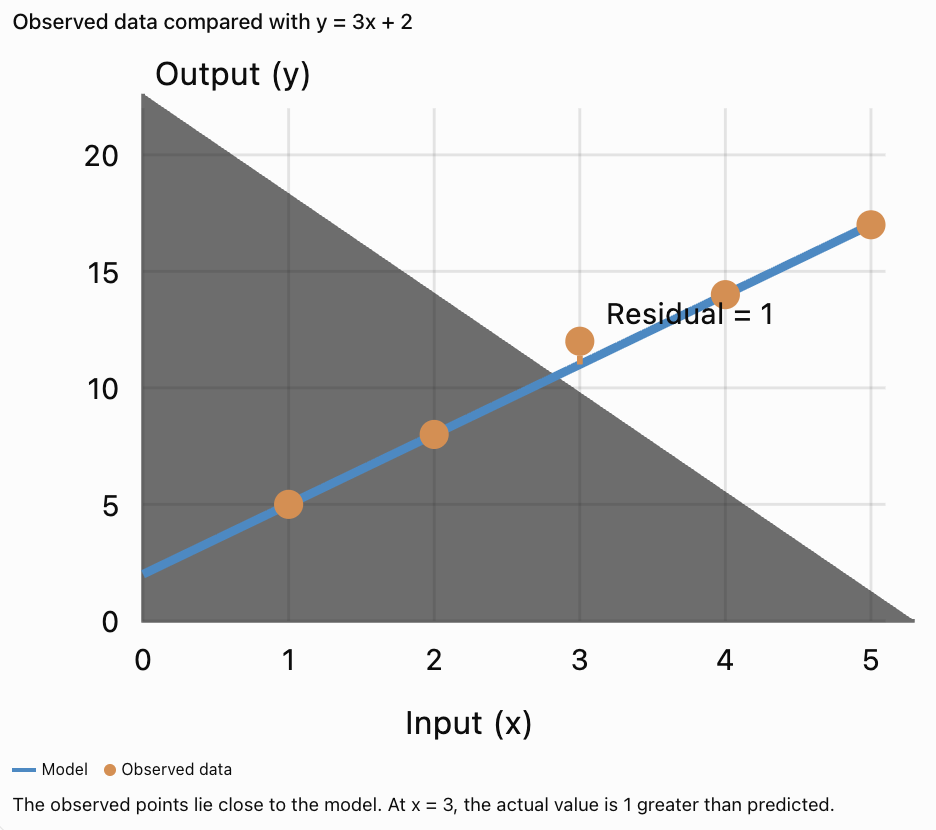
Suppose a model predicts:

y = 3x + 2

Most predictions match the observations exactly.

At x = 3, the model predicts 11 while the actual value is 12.

The difference is:

12 − 11 = 1

This difference is called a residual.

Residual Formula

Residual = Actual value − Predicted value

Interpretation

Small residuals may indicate a good fit, especially when compared with the scale of the measurements.

However, a single small residual does not prove that a model is reliable.

Visualising Model Fit

Interpolation and Extrapolation

Mathematical models can be used to predict values within or beyond the observed data.

Interpolation

Interpolation means estimating a value within the range of observed data.

For example, if measurements were collected between 0 and 10 minutes, predicting a value at 6 minutes is interpolation.

Extrapolation

Extrapolation means predicting a value outside the observed range.

For example, using the same data to predict a value at 50 minutes is extrapolation.

Important Observation

Extrapolation is often less reliable because the relationship may change outside the observed range.

Evaluating the Reasonableness of Predictions

A mathematical model should produce answers that make sense in context.

Example

A water tank begins with 100 litres and loses 5 litres per minute.

The model is:

V = 100 − 5t

After 10 minutes:

V = 100 − 5(10)

V = 50 L

This is reasonable.

After 30 minutes:

V = 100 − 5(30)

V = −50 L

A negative volume is not physically possible.

Interpretation

The model is only valid until the tank becomes empty.

Set V = 0:

0 = 100 − 5t

5t = 100

t = 20 minutes

The physically meaningful domain is:

0 ≤ t ≤ 20

Important Observation

A mathematically correct calculation can produce an unrealistic answer if the model is used outside its valid domain.

Assumptions and Limitations of Mathematical Models

Mathematical models simplify real-world situations.

A model may assume:

• Prices remain constant.

• Speed does not change.

• There are no unexpected fees.

• Measurements are accurate.

• Conditions remain stable.

• Relationships continue in the same pattern.

Questions to Ask

• Does the model match the available data?

• Is the rate of change constant?

• Are important variables missing?

• Is the prediction within the observed range?

• Are the units correct?

• Does the answer make practical sense?

• Could changing conditions affect the result?

Important Observation

A useful model does not have to be perfect, but its assumptions and limitations should be understood.

A General Method for Creating Mathematical Models

Common Mistakes

Using the wrong type of model

Not every relationship is linear.

Confusing independent and dependent variables

Clearly identify which quantity depends on the other.

Ignoring the initial value

Some models include a fixed starting amount.

Calculating the rate of change incorrectly

Use change in output divided by change in input.

Assuming all linear models are directly proportional

A linear model may have a nonzero initial value.

Failing to check known values

A model should agree with the data used to construct it.

Using unrealistic predictions

A model may not remain valid indefinitely.

Ignoring units

A rate may represent dollars per item, litres per minute, or kilometres per hour.

Confusing interpolation and extrapolation

Predictions beyond observed data require additional caution.

Assuming models are exact

Real-world measurements and relationships may contain uncertainty.

Key Terms

• Mathematical Model: Mathematical representation of a real-world situation.

• Algebraic Rule: Equation describing a relationship between variables.

• Variable: Symbol representing an unknown or changing quantity.

• Independent Variable: Input quantity.

• Dependent Variable: Output quantity.

• Linear Model: Model with a constant rate of change.

• Direct Variation: Relationship represented by y = kx.

• Rate of Change: Change in output divided by change in input.

• Slope: Rate of change of a linear relationship.

• Initial Value: Output when the input equals zero.

• y-Intercept: Point where a graph crosses the y-axis.

• Prediction: Estimate calculated using a model.

• Interpolation: Estimating within the observed data range.

• Extrapolation: Predicting beyond the observed data range.

• Residual: Difference between an actual value and its predicted value.

• Model Fit: How closely a model represents observed data.

• Assumption: Condition accepted as true when constructing a model.

• Limitation: Restriction affecting the accuracy or usefulness of a model.

• Domain: Set of permitted input values.

• Range: Set of possible output values.

• Verification: Checking whether a model agrees with known information.

• Proportional Relationship: Relationship where one quantity is a constant multiple of another.

• Nonlinear Relationship: Relationship without a constant rate of change.

Key Takeaways

• Mathematical models describe relationships between quantities.

• Algebraic rules can represent real-world situations.

• Variables represent quantities that can change.

• Linear models have the form y = mx + b.

• The slope describes the rate of change.

• The initial value represents the output when the input is zero.

• Direct variation is a special type of linear relationship.

• Tables and graphs can help identify mathematical patterns.

• Models can be used to predict unknown values.

• Equations can be rearranged to calculate inputs or outputs.

• Real-world models often depend on simplifying assumptions.

• A model should be checked against observed data.

• Residuals measure differences between observed and predicted values.

• Interpolation estimates within the observed range.

• Extrapolation predicts beyond the observed range.

• A model may be valid only within a particular domain.

• Predictions should be evaluated for reasonableness.

Check Your Understanding

Understanding Mathematical Models

1. What is a mathematical model?

2. What is the difference between an independent and dependent variable?

3. What does the slope represent in a linear model?

4. What does the initial value represent?

5. Why are mathematical models useful?

Creating Algebraic Rules

6. A notebook costs $5. Write an equation for the cost of n notebooks.

7. A taxi charges $4 initially plus $3 per kilometre. Write the equation.

8. A worker earns $20 per hour plus a $50 bonus. Write an equation for earnings.

9. A tank begins with 200 litres and loses 10 litres per minute. Write an equation for volume.

10. Find the rule for the points (0, 3), (1, 7), (2, 11), and (3, 15).

Making Predictions

11. If C = 4n + 6, find C when n = 8.

12. If V = 100 − 5t, find V when t = 12.

13. If E = 18h + 30, find E when h = 10.

14. If d = 60t, find d when t = 2.5.

15. If y = 3x + 7, find x when y = 28.

Evaluating Models

16. Why might a linear model fail to predict long-term population growth?

17. What is interpolation?

18. What is extrapolation?

19. What is a residual?

20. Why should mathematical predictions be checked for reasonableness?

Answer Key

Extended Challenge

1. A delivery company charges $8 plus $2.50 per kilometre. Construct a model and calculate the cost of a 24 km delivery.

2. A tank contains 500 litres and loses 15 litres per minute. Write a model and determine when it becomes empty.

3. A worker earns $22 per hour plus a $75 bonus. Write a model and determine earnings after 16 hours.

4. Find the linear equation passing through (3, 14) and (7, 30).

5. A machine produces 180 items in 6 minutes at a constant rate. Construct a model for production.

6. Two companies charge C₁ = 4x + 25 and C₂ = 6x + 5. Determine when their costs are equal.

7. A model predicts y = 5x + 2. If the actual value at x = 4 is 25, calculate the residual.

8. Explain why a linear model may be unsuitable for a population that doubles every year.

9. A liquid cools from 90°C to 70°C in 5 minutes. Assuming a constant cooling rate over a short interval, construct a model.

10. Describe three factors that might limit the accuracy of a mathematical model.

Final Investigation: Comparing School Transport Options

A school is planning transportation for an educational trip.

Two bus companies offer different pricing structures.

Company A

• Fixed booking fee: $80

• Cost per student: $6

Company B

• Fixed booking fee: $140

• Cost per student: $4

Part A: Constructing Models

1. Identify the independent variable.

2. Identify the dependent variable.

3. Write an equation for Company A.

4. Write an equation for Company B.

5. Identify the slope and initial value of each equation.

Part B: Making Predictions

6. Calculate the cost for 10 students using each company.

7. Calculate the cost for 20 students.

8. Calculate the cost for 30 students.

9. Calculate the cost for 40 students.

10. Organise the results in a table.

Part C: Comparing Models

11. Graph both equations.

12. Determine which company has the lower starting fee.

13. Determine which company has the lower cost per student.

14. Calculate the number of students at which both companies charge the same amount.

15. Determine the cost at that number of students.

Part D: Evaluating the Models

16. Determine which company is cheaper for 50 students.

17. Calculate the difference in cost for 50 students.

18. Explain which company is more suitable for smaller groups.

19. Identify two assumptions made by these pricing models.

20. Write a conclusion explaining how mathematical models help schools make informed decisions.

Investigation Check

Company A

C = 6n + 80

Company B

C = 4n + 140

Equal Costs

6n + 80 = 4n + 140

2n = 60

n = 30 students

At 30 students:

C = 6(30) + 80

C = $260

For 50 Students

Company A:

C = 6(50) + 80 = $380

Company B:

C = 4(50) + 140 = $340

Company B is cheaper by $40.

Conclusion

Company A is cheaper for fewer than 30 students. Both companies charge the same amount for 30 students. Company B is cheaper for more than 30 students.